6.4: Closed-Loop Frequency Response

Closed-Loop Frequency Response

The closed-loop frequency response reveals important information about the relative stability and the speed of response in the time-domain. For unity-gain feedback configuration \((H(s)=1)\), the closed-loop frequency response is computed as:

\[T(j\omega )=\dfrac{KG(j\omega )}{1+KG(j\omega )} \nonumber \]

To proceed further, we use rectangular form expression for the open loop frequency response: \(KG(j\omega )=X(j\omega )+jY(j\omega )\); then,

\[T(j\omega )=\dfrac{X+jY}{\left(1+X\right)+jY} =Me^{j\phi } \nonumber \]

and

\[\left|T(j\omega )\right|^{2} =\dfrac{X^{2} +Y^{2} }{\left(1+X\right)^{2} +Y^{2} } =M^{2}. \nonumber \]

The latter can be rearranged to obtain:

\[\left(X+\frac{M^{2} }{M^{2} -1} \right)^{2} +Y^{2} =\dfrac{M^{2} }{(M^{2} -1)^{2} } . \nonumber \]

The above relation represents the equation of a circle with center at \(X=\frac{M^{2} }{1-M^{2} } ,\, \, Y=0\), and radius \(r=\frac{M}{1-M^{2} }\); these are described as constant \(M\) circles on the frequency response plot. Further, as \(M\to 1,\, \, X=-\frac{1}{2}\), which is a vertical line that separates the circles for \(M<1\) from those with \(M>1\).

The phase relationship similarly reveals an equation for constant phase circles:

\[\left(X+\frac{1}{2} \right)^{2} +\left(Y-\frac{1}{2N} \right)^{2} =\frac{1}{4} +\left(\frac{1}{2N} \right)^{2} \nonumber \]

where \(N=\tan \phi\). The constant phase circles are centered at: \(X=-\frac{1}{2} ,\, \, Y=\frac{1}{2N}\), and have radius: \(r=\sqrt{\frac{1}{4} +\left(\frac{1}{2N} \right)^{2} }\).

Resonance Peak 

The resonance peak in the frequency response occurs at \(\omega =\omega _{r}\) for \(\zeta <0.7\). In particular, for a prototype second-order system, we have:

Resonant frequency: \(\omega _{r} =\omega _{n} \sqrt{1-2\zeta ^{2} }\)

Resonant peak: \(M_{r} =\left|T(j\omega _{r} )\right|=\frac{1}{2\zeta \sqrt{1-\zeta ^{2} } }\)

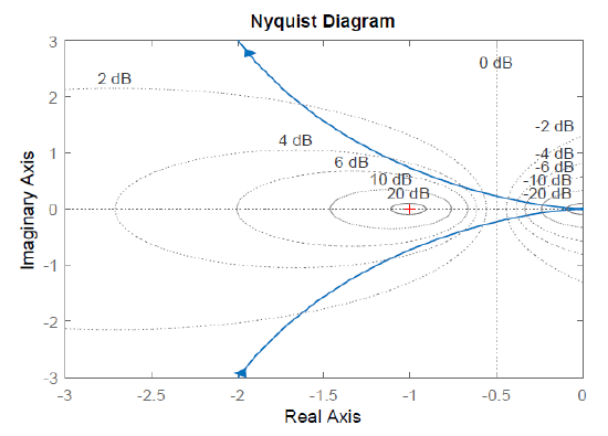
When the polar plot of the loop gain, \(KGH(j\omega )\), is superimposed onto the constant \(M\) and constant \(N\) contours, it reveals the magnitude peak \(M_{r}\) in \(T(j\omega )\).   The MATLAB Control System Toolbox 'grid' command adds constant \(M,N\) contours on the Nyquist plot.

The resonance peak in the closed-loop frequency response represents a measure of relative stability; the resonant frequency serves as a measure of speed of response in the time-domain. A value of \(M_{r} =1.3\)\((or\ 2.5dB)\) is considered a good compromise between speed and stability.

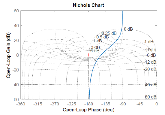
The Nichol’s Chart

The closed-loop frequency response can be alternately visualized on the Nichol’s chart, where the magnitude in dB is plotted along the vertical axis, and the phase in degrees is plotted along the horizontal axis.

The MATLAB Control System Toolbox 'grid' command similarly adds constant \(M,N\) contours on the Nichol's chart.

Example \(\PageIndex{1}\)

Let  \(KG(s)=\frac{10}{s(s+1.86)}\), \(KG(j\omega )=\frac{10}{-\omega ^{2} +j1.86\omega } \);

then, the closed-loop frequency response has a peak \(M_{r} =5\; \rm dB\), as can be observed on both the Nyquist plot and Nichol’s chart  in Figure 6.4.1 (an imaginary \(5\rm dB\) circles touches the \(KG(j\omega )\) curve).

Figure \(\PageIndex{1}\): Closed-loop frequency response evaluation on the Nyquist plot (left) and Nichol’s chart (right).