7.3: Sampled-Data System Response
- Page ID
- 24419

The response of a sampled-data system, \(G\left(z\right)\), to an input sequence, \(u\left(k\right)\), is the output sequence, \(y(k)\). In the \(z\)-domain, the system response is given as: \(y\left(z\right)=G\left(z\right)u(z)\).
Alternatively, we may use inverse z-transform to obtain an input–output description in the form of a difference equation that can be solved by iteration.
7.3.1 Difference Equation Representation
Let \(G\left(z\right)=\frac{n\left(z\right)}{d\left(z\right)},\) where \(n\left(z\right)\) and \(d\left(z\right)\) are \(m\)th order and \(n\)th order polynomials, given as:
\[n\left(z\right)=\sum^m_{i=0}{b_iz^{m-i}},\ \ d\left(z\right)=z^n+\sum^n_{i=1}{a_iz^{n-i}}. \nonumber \]
Then \(d\left(z\right)y\left(z\right)=n\left(z\right)u\left(z\right)\). By applying the inverse \(z\)-transform, we obtain a difference equation, described as:
\[y\left(k+n\right)+\sum^n_{i=1}{a_iy\left(k+n-i\right)}+\sum^m_{i=0}{b_iu\left(k+m-i\right)} \nonumber \]
As the system is linear and time-invariant, we apply a time shift and rearrange the difference equation into and update rule:
\[y\left(k\right)=-\sum^n_{i=1}{a_iy\left(k-i\right)}+\sum^m_{i=0}{b_iu\left(k-i\right)} \nonumber \]
The above rule can be programmed on a computer to solve for the response of the sampled-data system to an input sequence, \(u\left(k\right)\), described as: as \(u\left(k\right)={\left.u\left(t\right)\right|}_{t=kT}\).
Let \(G(z)=\frac{y(z)}{u(z)} =\frac{0.181}{z-0.819}\); then, the sampled-data system is described by the following input–output relation:
\[y\left(k\right)=0.819y\left(k-1\right)+0.181u\left(k-1\right) \nonumber \]
Let \(G(z)=\frac{0.0187(z+0.936)}{(z-1)(z-0.819)}\); then, the sampled-data system is described by the following input–output relation:
\[y\left(k\right)=1.819y\left(k-1\right)-0.819y\left(k-2\right)+0.0187u\left(k-1\right)+0.0175u(k-2) \nonumber \]
Unit-Pulse Response
The unit-pulse response of a sampled-data system model, \(G(z)\), is its response to a unit-pulse \(r(k)=\delta (k)\).
Using \(r\left(z\right)=1\), the unit-pulse response is computed as: \(g\left(kT\right)=z^{-1}\left[G(z)\right]\), with an implicit sampling time \(T=1s\).
Unit-pulse response for sample time, \(T\), is obtained by assuming \(\delta \left(z\right)=\frac{1}{T}\), hence \(g\left(kT\right)=\frac{1}{T}z^{-1}\left[G(z)\right]\).
Alternatively, given the input–output description, the unit-pulse response can be computed by iteration.
The unit-pulse response comprises the natural response modes \(G\left(z\right)=n(z)/d\left(z\right)\). These modes depend on the roots of \(d\left(z\right)\), and are characterized as follows:
Real Roots. Assume that \(d\left(z\right)\) has real and distinct roots: \(z_{i} ,\; i=1,\ldots ,n,\)then, the natural response modes are given as: \(\phi _{i} (k)=(z_{i} )^{k}\). These modes die out with time if \(|z_{i} |<1.\)
Complex Roots. Assume that \(d\left(z\right)\) has complex roots of the form: \(re^{\pm j\theta }\); then, its natural response modes are given as: \(\phi _{i} (k)=\{ r^{k} \; \cos k\theta ,\; r^{k} \; \sin k\theta \}\). These modes similarly die out with time if \(|r|<1\).
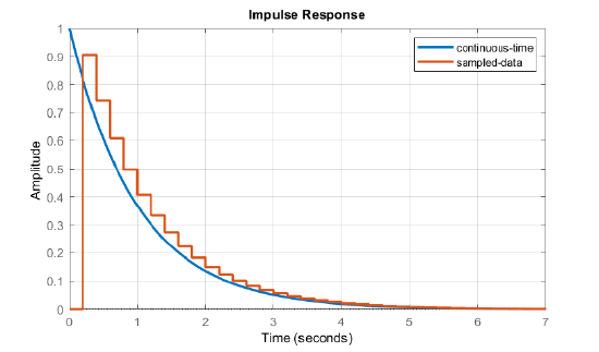
Let \(G(s)=\frac{1}{s+1}\); use \(T=0.2\rm s\) to obtain: \(G(z)=\frac{0.181}{z-0.819}\). The sampled-data system is described by the following input-output relation: \(y\left(k\right)=0.819y\left(k-1\right)+0.181u\left(k-1\right).\)
As \(T=0.2s\), let \(\delta \left(k\right)=\{5,\ 0,\ 0,\dots \}\); then, assuming zero initial conditions, the unit-pulse response is obtained as:
\[y\left(k\right)=\left\{0,0.906,\ 0.742,\ 0.608,\ 0.497,0.407,\ 0.333,\ \dots \right\} \nonumber \]
For comparison, the impulse response of the analog system is obtained as: \(g\left(t\right)=e^{-t}u(t)\).
The impulse responses of continuous and discrete systems are compared in Figure 7.3.1.
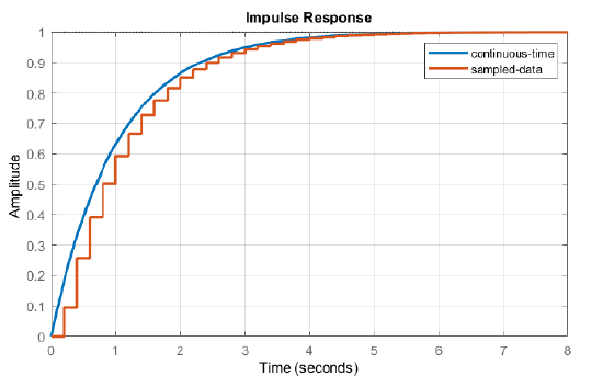
Let \(G(s)=\frac{1}{s(s+1)}\); use \(T=0.2\rm s\) to obtain: \(G(z)=\frac{0.0187(z+0.936)}{(z-1)(z-0.819)}\). The sampled-data system is described by the following input-output relation:
\[y\left(k\right)=1.819y\left(k-1\right)-0.819y\left(k-2\right)+0.0187u\left(k-1\right)+0.0175u(k-2). \nonumber \]
Assuming \(u\left(k\right)=\{5,0,0,\dots \}\), and zero initial conditions, the unit-pulse response is obtained as:
\[y\left(k\right)=\left\{0,0.0937,\ 0.258,\ 0.392,\ 0.502,0.593,\ 0.667,\ \dots \right\} \nonumber \]
For comparison, the impulse response of the original analog system is obtained as: \(g\left(t\right)=(1-e^{-t})u(t)\).
The impulse responses of continuous and discrete systems are compared in Figure 7.3.2. We note that the presence of integrator in the transfer function causes the impulse response to asymptotically approach unity in the steady-state.
In the MATLAB Control Systems Toolbox, the ‘impulse’ command can be used to obtain or plot the unit-pulse response of a sampled-data system.
Unit-Step Response
The unit-step response of a sampled-data system model, \(G\left(z\right)\), is its response to the unit-step sequence: \(r\{ kT\} =\{ 1,1,1\ldots \}\); \(r(z)=\frac{1}{1-z^{-1} }\). In the \(z\)-domain, the unit-step response is obtained as: \(y(z)=\frac{G(z)}{1-z^{-1} }\).
Alternatively, using the input-output system description, the unit-step response can be obtained by iteration.
Let \(G(s)=\frac{1}{s+1}\); use \(T=0.2\rm s\) to obtain: \(G(z)=\frac{0.181}{z-0.819}\). The unit-step response is computed as:\(y(z)=\frac{0.181z}{\left(z-1\right)\left(z-0.819\right)}\).
We use PFE of \(y(z)/z\) to obtain: \(y(z)=\left(\frac{z}{z-1} -\frac{z}{z-0.819} \right).\)Using the inverse \(z\)-transform, the step response sequence is obtained as: \(y(kT)=1-(0.819)^{k} ,\; \; k=0,1,\ldots\)
Alternatively, we use the input-output system description with zero initial conditions: \(y\left(k\right)=0.819y\left(k-1\right)+0.181u\left(k-1\right).\) The resulting unit-step sequence is given as: \(y\left(k\right)=\left\{0,\ 0.181,\ 0.329,\ 0.451,\ 0.55,\dots \right\}\).
For comparison, the unit-step response of continuous-time system is given as:\(y(t)=1-e^{-t} ,\; \; t>0.\) The step responses of the continuous and discrete systems are plotted alongside (Figure 7.3.3).
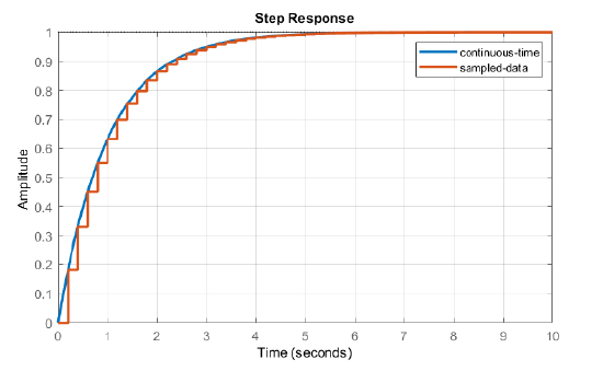
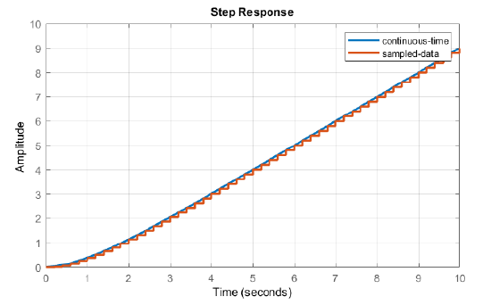
Let \(G(s)=\frac{1}{s(s+1)}\); use \(T=0.2\rm s\) to obtain: \(G(z)=\frac{0.0187z+0.0175}{z^{2} -1.819z+0.819}\). Using the time-domain relation (Example 6.8), the unit-step response is given as: \(\{ 0,\; \; 0.0187,\; 0.0702,\; 0.149,\, 0.249,\, 0.368,\, 0.501,0.647,0.802,0.965,\ldots \}\)
Analytically, let \(r(z)=\frac{z}{z-1}\) (unit-step); then, the system output is given as: \(y(z)=\frac{z(0.0187z+0.0175)}{(z-1)(z^{2} -1.819z+0.819)}\). By using long division, we can express the quotient as:
\[y(z)=0.0187z^{-1} +0.0703z^{-2} +0.149z^{-3} +0.249z^{-4} +0.501z^{-5} +\ldots \nonumber \]
The resulting output sequence matches the one obtained by iteration.
For comparison, continuous-time system step response is given as: \(y(t)=(t-1+e^{-t} )u(t).\)
The step responses of the continuous and discrete systems are plotted alongside (Figure 7.3.4).
In the MATLAB Control Systems Toolbox, the ‘step’ command can be used to obtain or plot the unit-step response of a sampled-data system.
Response to Arbitrary Inputs
Given the unit-pulse response of the system, its response to an arbitrary input sequence is obtained by convolution. Accordingly, let the unit-pulse response sequence be given as:
\[\left\{g\left(k\right)\right\}=\{g\left(1\right),\ g\left(2\right),\ \dots \} \nonumber \]
Then, using an arbitrary input sequence: \(\left\{u\left(k\right)\right\}=\{u\left(1\right),\ u\left(2\right),\ \dots \}\), the output sequence is given by the convolution sum:
\[y\left(k\right)=g\left(k\right)*u\left(k\right)=\sum^{\infty }_{i=0}{g\left(k-i\right)u\left(i\right)} \nonumber \]
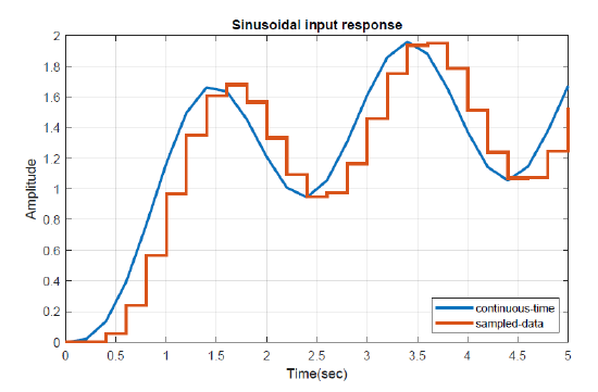
As an example, we obtain the output for a sinusoidal input below.
Let \(G(z)=\frac{0.368z+0.264}{(z-1)(z-0.368)}\); we assume a sinusoidal input sequence, \(u\left(kT\right)={sin \left(\pi kT\right)\ }\). Then, the output response is computed using the convolution sum is shown (Figure 7.3.5).