
7.5: Closed-Loop System Response
- Page ID
- 24421

Closed-Loop System Step Response
We consider a unity-gain feedback sampled-data control system (Figure 7.1), where an analog plant is driven by a digital controller through a ZOH.
Let the pulse transfer function be given as: \(G\left(z\right)=\frac{n\left(z\right)}{d\left(z\right)}\)
Then, for a static controller, the closed-loop pulse transfer function in unity-feedback configuration is defined as:
\[T(z)=\frac{Kn(z)}{d(z)+Kn(z)} . \nonumber \]
Given the closed-loop pulse transfer function, \(T(z)\), we compute its response to a unit-step sequence, \(r\left(kT\right)=\{1,1,\dots \}\).
The response can be obtained by iteration, or analytically from the expression: \(y\left(z\right)=T\left(z\right)r\left(z\right)\).
Let \(G(s)=\frac{1}{s+1}\), \(T=0.2\; \rm s\); then, we have \(G(z)=\frac{0.181}{z-0.819}\)
The closed-loop pulse transfer function is given as: \(T(z)=\frac{0.6181K}{z-0.819+0.181K}. \nonumber\)
Let \(K=1\), and assume \(r(kT)=1,\; \; r(z)=\frac{1}{1-z^{-1} }\); then, system response is obtained as: \(y(z)=\frac{0.181z}{(z-1)(z-0.638)} . \nonumber \)
Using PFE, \(y(z)=0.5\left(\frac{z}{z-1} -\frac{z}{z-0.638} \right). \nonumber\)
The resulting output sequence is given as: \(y(kT)=0.5(1-0.638^{k} ),\; \; k=0,1,\ldots\)
or \(y\left(k\right)= \{ 0,\; \; 0.632,\; 0.465,\; 0.509,\, 0.498,\, 0.501,\, 0.5,\, 0.5\ldots \}. \nonumber\)
For comparison, for \(K=1\), the analog system response is given as: \(y(t)=\frac{1}{2} (1-e^{-2t} ),\; \; t>0. \nonumber\)
The step responses are compared in Figure 7.5.1.

Let \(G(s)=\frac{1}{s(s+1)}\), \(T=0.2\rm s\); then, we obtain: \(G(z)=\frac{0.0187z+0.0175}{(z-1)(z-0.819)}. \nonumber\)
The closed-loop pulse transfer function is: \(T(z)=\frac{(0.0187z+0.0175)K}{(z-1)(z-0.819)+(0.0187z+0.0175)K} \nonumber\)
Let \(K=1;\) then, the closed-loop pulse transfer function is: \(T(z)=\frac{0.0187z+0.0175}{z^{2} -1.8z+0.836}. \nonumber\)
Let \(r(z)=\frac{z}{z-1}\) (unit step); then, the closed-loop system response is given as: \(y(z)=\frac{z\left(0.0187z+0.0175\right)}{\left(z-1\right)\left(z^{2} -1.8z+0.836\right)}. \nonumber\)
By using long division, we obtain: \(y(z)=0.368z^{-1} +z^{-2} +1.4z^{-3} +1.4z^{-4} +1.15z^{-5} +\ldots \nonumber\)
The step response sequence is given as: \(y(kT)=\{ 0,\; 0.368,\; 1,\; 1.4,\; 1.4,\; 1.15,\; \ldots \}\)
For comparison, the analog system has a closed-loop transfer function: \(T(s)=\frac{1}{s^{2} +s+1} \nonumber.\)
Its unit-step response is obtained as: \(y(t)=(1-1.15e^{-0.5t} \sin 0.866\, t)u(t). \nonumber\)
The step responses are compared in Figure 7.5.2.
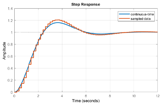
From the comparison of step responses, we observe that the analog system response has a \(16.3\%\) overshoot, whereas the discrete system response has a higher (\(18\%\)) overshoot. The discrete system also has a higher settling time compared to the analog system.
The higher overshoot in the case of sampled-data system occurs due to the negative phase contributed by the ZOH that reduces the available phase margin by an amount: \(\Delta \phi _\rm m =\frac{\omega _{{\rm g}c} T}{2} .\)
In particular, from the MATLAB ‘margin’ command, the continuous-time system has a PM of \(52^{\circ }\) at \(\omega _{\rm gc} =0.786\; \frac{\rm rad}{\rm s}\). Since \(T=0.2 \;\rm sec\), the reduction is phase margin is: \(\Delta \phi _\rm m =4.5^{\circ }\).
Steady-State Tracking Error
The tracking error, \(e(z),\) in response to a given reference input \(r(z),\) in the case of a unity-gain feedback sampled-data system is computed as:
\[e(z)=r(z)(1-T(z)). \nonumber \]
The final value theorem (FVT) in the \(z\)-domain is stated as:
\[{\mathop{\lim }\limits_{k\to \infty }} e(k)\; ={\mathop{\lim }\limits_{z\to 1}} (z-1)e(z).\; \nonumber \]
The position and velocity error constants in the case of sampled-data system are defined as:
\[K_\rm p ={\mathop{\lim }\limits_{z\to 1}} G(z)\; \nonumber \]
\[K_{\rm v} ={\mathop{\lim }\limits_{z\to 1}} \frac{(z-1)}{T} G(z)\; \nonumber \]
Using the error constants, the steady-state errors to step and ramp inputs are computed as:
\[\left. e_{\rm ss} \right|_{\rm step} =\frac{1}{1+K_\rm p } \nonumber \]
\[\left. e_{\rm ss} \right|_{\rm ramp} =\frac{1}{K_{\rm v} } . \nonumber \]
Let \(G(z)=\frac{0.0187z+0.0175}{(z-1)(z-0.819)} \, \, \left(T=0.2s\right) \nonumber\); then, the error constants are given as \(K_\rm p =\infty\) and \(K_{\rm v} =1\).
Accordingly, \(\left. e_{\rm ss} \right|_{\rm step} =0;\; \left. e_{\rm ss} \right|_{\rm ramp} =0.2. \nonumber\)
Let \(G(z)=\frac{0.368z+0.264}{(z-1)(z-0.368)} \nonumber\) with \(T=1\rm s\); then, we have \(K_\rm p =\infty ,\; \; K_{\rm v} =1. \nonumber\)
Accordingly, \(\left. e_{\rm ss} \right|_{\rm step} =0;\; \left. e_{\rm ss} \right|_{\rm ramp} =1. \nonumber\)