7.6: Digital Controller Design by Emulation
- Page ID
- 24422

Emulation of Analog Controllers
A controller for a sampled-data control system can be obtained by emulating (i.e., approximating) an available analog controller design. Controller emulation aims to obtain an approximate digital controller, \(K\left(z\right)\), whose response matches that of the analog controller, \(K\left(s\right)\) as measured by a selected metric.
Popular controller emulation methods include:
Impulse Invariance. The impulse invariance method of digital controller design aims to match the impulse response of the analog controller. Assume that the analog controller is of the form: \(K(s)=\sum _{k=1}^{n} \frac{A_{k} }{s-s_{k} }\). Then, a corresponding digital controller is obtained as: \(K(z)=T\sum _{k=1}^{n} \frac{A_{k} }{1-p_{k} z^{-1} } ,\quad p_{k} =e^{s_{k} T} ,\) that is, the controller poles are mapped to their respective locations in the \(z\)-plane.
Pole–Zero Matching. In pole–zero matching, both the plant poles and zeros are mapped to their equivalent locations in the \(z\)-plane using: \(z_{i} =e^{s_{i} T}\). If the analog controller transfer function has \(n\) poles and \(m\) finite zeros, to be matched, then another \(n-m\) zeros are added at \(z=1\). Additionally, the dc gain of the digital controller is matched to that of the analog controller.
Zero-Order Hold (ZOH). The ZOH method assumes the presence of a ZOH at the input to the controller. The method is ineffective if the analog controller has poles at the origin (as in the case of PI and PID controllers).
First-Order Hold (FOH). The FOH method assumes a piece-wise linear input to the controller.
Bilinear Transform (BLT). The BLT method uses Tustin’s approximation \(\left(z\cong \frac{1+Ts/2}{1-Ts/2}\right)\) to emulate an analog controller. The BLT method is quite effective when used with a high sampling frequency. Using the BLT, an equivalent digital controller is obtained as: \(K(z)=K(s){\mathop{|}\nolimits_{s=\frac{2}{T} \, \frac{z-1}{z+1} }} .\)
The ‘c2d’ command in the MATLAB Control Systems Toolbox allows controller emulation method to be specified. The default method is ZOH.
Let \(G\left(s\right)=\frac{10}{s\left(s+2\right)(s+5)},\ T=0.2s\); then, the pulse transfer function is obtained as: \(G\left(z\right)=\frac{0.0095\left(z+0.18\right)\left(z+2.68\right)}{\left(z-1\right)\left(z-0.67\right)\left(z-0.37\right)}\)
A lead-lag controller for this example was designed earlier: \(K\left(s\right)=25\left(\frac{s+2}{s+24}\right)\left(\frac{s+0.05}{s+0.004}\right)\).
We use MATLAB Control System Toolbox ‘c2d’ commands to obtain discrete approximations of the controller using the following methods:
ZOH: \(K\left(z\right)=\frac{25\left(z-0.99\right)\left(z-0.925\right)}{\left(z-0.999\right)\left(z-0.008\right)}\)
FOH: \(K\left(z\right)=\frac{6.86\left(z-0.99\right)\left(z-0.7\right)}{\left(z-0.999\right)\left(z-0.008\right)}\)
BLT: \(K\left(z\right)=\frac{8.86\left(z-0.99\right)\left(z-0.667\right)}{\left(z-0.999\right)\left(z-0.412\right)}\)
Impulse-invariance: \(K\left(z\right)=\frac{-109.77z\left(z-0.999\right)}{\left(z-0.999\right)\left(z-0.008\right)}\)
Pole-zero matching: \(K\left(z\right)=\frac{6.3\left(z-0.99\right)\left(z-0.67\right)}{\left(z-0.999\right)\left(z-0.008\right)}\)
Least-squares: \(K\left(z\right)=\frac{5.74\left(z-0.99\right)\left(z-0.542\right)}{\left(z-0.999\right)\left(z-0.376\right)}\)
An analysis of the closed-loop systems shows that all except the impulse invariance approximation are stable with damping in the range of \(\zeta \in [0.72,0.81]\). The closed-loop responses are compared in Figure 7.6.1.
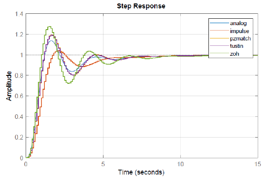
As seen from the figure and otherwise, the BLT method generally provides the best approximation of an analog controller.
Emulation of Analog PID Controller
An analog PID controller with input \(e(t)\) and output \(u(t)\) is described as:
\[u(t)=k_ p e(t)+k_ d \frac{ de(t)}{ dt} +k_{i} \int e(t) dt. \nonumber \]
An equivalent digital PID controller can be obtained by employing a forward Euler approximation of the derivative term: \(\frac{d}{dt}e\left(t\right)\approx \frac{1}{T}(e_{k+1}-e_k)\).
The resulting \(z\)-domain transfer functions for the PID controller are given as:
\[K\left(z\right)=k_p+k_d\left(\frac{z-1}{T}\right)+k_i\left(\frac{T}{z-1}\right) \nonumber \]
Further, let \(v_{k}\) denote the integrator output; then, the digital PID controller is implemented using the following update rules:
\[u_k=k_pe_{k-1}+\frac{1}{T}\left(e_k-e_{k-1}\right)+k_iv_k \nonumber \]
\[v_k=v_{k-1}+Te_{k-1} \nonumber \]
Let \(G\left(s\right)=\frac{10}{s\left(s+2\right)(s+5)},\ T=0.2s\); then, the pulse transfer function is obtained as: \(G\left(z\right)=\frac{0.0095\left(z+0.18\right)\left(z+2.68\right)}{\left(z-1\right)\left(z-0.67\right)\left(z-0.37\right)}\)
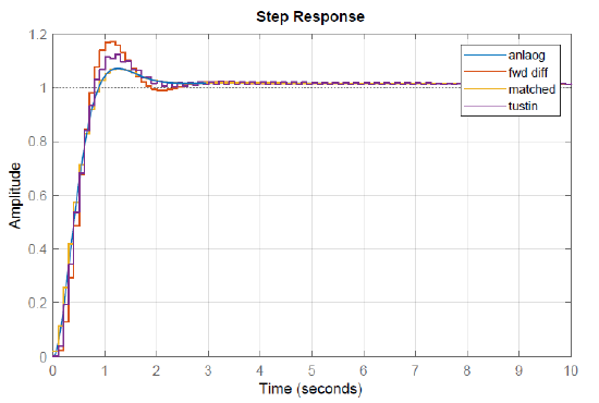
A PID controller for this example was designed earlier as: \(K_{PID}\left(s\right)=\frac{1.2\left(s+0.05\right)\left(s+2\right)}{s}\).
An approximate digital controller is obtained as: \(K_{PID}\left(z\right)=2.46+1.2\left(\frac{z-1}{T}\right)+0.12\left(\frac{T}{z-1}\right)\).
The step response of the closed-loop system for analog and digital PID controllers is shown in Figure 7.6.2. The discrete PID controller with forward Euler approximation of derivative emulates the analog controller well. However, pole-zero matching is seen to give the best result in this example.