
9.1: Controller Design in Sate-Space
- Page ID
- 24429

State Feedback Controller Design
The state feedback controller design refers to the selection of individual feedback gains for the complete set of state variables. It is assumed that all the state variables are available for observation. The design goal is to improve the transient response of the system and reduce the steady-state tracking error.
Let \({\bf x}(t)\) denote a vector of \(n\) state variables, \(u(t)\) denote a scalar input, and \(y(t)\) denote a scalar output; then the state variable model of a SISO system is given as: \[\dot{\bf x}(t)={\bf Ax}(t)+{\bf b}u(t), \;\; y(t)={\bf c}^{T} {\bf x}(t) \nonumber \]
where \({\bf A}\) is a \(n\times n\) system matrix, \({\bf b}\) is a \(n\times 1\) column vector, and \({\bf c}^{T}\) is a \(1\times n\) row vector. The above state variable model represents a strictly proper input-output transfer function.
Controller design in state-space involves selection of suitable feedback gain vector, \({\bf k}^T\), that imparts desired stability and performance characteristics to the closed-loop system.
Pole Placement Design
Pole placement design refers to the selection of the feedback gain vector that places the poles of the characteristic polynomial at the desired locations. The control law for the pole placement design is expressed as: \[u(t)=-{\bf k}^{T} {\bf x}(t)+r(t), \nonumber \]
where \({\bf k}^{T} =[k_{1} ,\; \; k_{2} ,\; \ldots ,k_{n} ]\) is a vector of \(n\) feedback gains, one for each of the \(n\) state variables, and \(r(t)\) is a reference input.
A necessary condition for pole placement using state feedback is that pair \(\left({\bf A,\,b}\right)\) is controllable, i.e., its controllability matrix, \({\bf M}_{\rm C}\), is of full rank, where \({\bf M}_{\rm C} =[{\bf b,\; Ab,\;\ldots ,\;A}^{n-1} {\bf b}]\) .
By including control law in the state equations, the closed-loop system is given as:
\[\dot{\bf x}(t)=({\bf A-bk}^{T}){\bf x}(t)+{\bf b}r(t) \nonumber \]
The design problem, then, is to select the feedback gain vector \({\bf k}^T\) that multiplies the state vector \({\bf x}(t)\), such that the closed-loop system matrix \({\bf A-bk}^{T}\) has characteristic polynomial that aligns with a desired polynomial, i.e.,
\[\left|s{\bf I-A+bk}^{T} \right|=\Delta _{\rm des} (s) \nonumber \]
The above equation relates two \(n\)th order polynomials; by equating the polynomial coefficients on both sides of the equation, we obtain \(n\) linear equations that can be solved for the \(n\) feedback gains: \(k_{i} ,\; i=1,\ldots ,n\).
The desired characteristic polynomial for pole placement design is selected with root locations that meet the time-domain performance criteria.
Closed-loop System
The closed-loop system model is given as: \[\dot{\bf x}(t)={\bf A}_{\rm cl}{\bf x}(t)+{\bf b}r(t) \nonumber \]
where \({\bf A}_{\rm cl} =({\bf A-bk}^{T})\). Assuming closed-loop stability, for a constant input \(r(t)=r_{\rm ss}\), the steady-state response, \({\bf x}_{\rm ss}\), obeys:
\[0 ={\bf A}_{\rm cl} {\bf x}_{ss} +{\bf b} r_{ss} ,\;\; y_{\rm ss} ={\bf c}^T {\bf x}_{ss} \nonumber \]
Hence, \(y_{\rm ss}={\bf c}^T\,{\bf A}_{\rm cl}^{-1}\,{\bf b}\,r_{\rm ss}\).
The state and output equations for a DC motor model are given as:
\[\frac{\rm d}{\rm dt} \left[\begin{array}{c} {i_a } \\ {\omega } \end{array}\right]=\left[\begin{array}{cc} {-100} & {-5} \\ {5} & {-10} \end{array}\right] \left[\begin{array}{c} {i_a } \\ {\omega } \end{array}\right]+\left[\begin{array}{c} {100} \\ {0} \end{array}\right]V_a , \;\;\omega =\left[\begin{array}{cc} {0} & {1} \end{array}\right]\left[\begin{array}{c} {i_a } \\ {\omega } \end{array}\right]. \nonumber \]
The motor model has a denominator polynomial \(\Delta (s)=s^{2} +110s+1025\); its roots are located at \(s_{1,2} =-10.28,\; -99.72\) that are reciprocals of the motor time constants \((\tau _\rm e \cong 10\; \rm msec,\; \tau _\rm m \cong 100\; \rm msec)\).
Assume that the design specifications require the closed-loop response to have a time constant of \(20ms\).
To reduce a time constants to \(20\; \rm msec\), we may choose to place the closed-loop poles at \(-50\),\(-100\). Then, the desired characteristic polynomial is given as: \(\Delta _{\rm des} (s)=s^{2} +150s+5000\).
We may assume \(r=0\), so the control law is given as: \(V_a =-k^{T} x\), where \(k^{T} =[k_{1} ,\;k_{2} ]\).
With the inclusion of state feedback, the closed-loop system matrix is given as:
\[A-bk^{T} =\left[\begin{array}{cc} {-100(1+k_{1} )} & {-5(1+20k_{2})} \\ {5} & {-10} \end{array}\right] \nonumber \]
The closed-loop characteristic polynomial is given as:
\[\left|sI-A+bk^{T} \right|=(s+10)\left[s+100(1+k_{1} )\right]+25(1+20k_{2} ). \nonumber \]
By comparing the coefficients of the two polynomials, we obtain the feedback gains: \(k_{1} =0.4,k_{2} =7.15\). The resulting control law is given as:
\[V_a\left(t\right)=-0.4\ i_a\left(t\right)-7.15\ \omega (t) \nonumber \]
The closed-loop system system matrix is given as: \(\left[\begin{array}{cc} {-140} & {-20} \\ {5} & {-10} \end{array}\right]\).
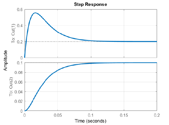
The steady-state system response is given as: \(y_{\rm ss}=0.1r_{\rm ss}\).
The step response of the closed-loop system is plotted in Figure \(\PageIndex{1}\).
Pole Placement in Controller Form
The pole placement design is facilitated if the system model is in the controller form (Section 8.3.1). In the controller form structure, the coefficients of the characteristic polynomial appear in reverse order in the last row of \(A\) matrix.
\[A=\left[\begin{array}{cc} {\begin{array}{cc} {0\; \; \; \; \; \; \; } & {1} \\ {0\; \; \; \; \; \; \; } & {0} \end{array}} & {\begin{array}{cc} {0\; \; \; } & {\ldots } \\ {1\; \; \; } & {\ldots } \end{array}} \\ {\begin{array}{cc} {\; \; \; \vdots } & {\vdots } \\ {-a_{n} } & {-a_{n-1} } \end{array}} & {\begin{array}{cc} {\ddots } & {1} \\ {\ldots } & {-a_{1} } \end{array}} \end{array}\right],\quad b=\left[\begin{array}{c} {\begin{array}{c} {0} \\ {0} \end{array}} \\ {\begin{array}{c} {\vdots } \\ {1} \end{array}} \end{array}\right]. \nonumber \]
Then, using full state feedback through \(u=-k^{T} x+r\), the closed-loop system matrix is given as:
\[A-bk^{T} =\left[\begin{array}{cc} {\begin{array}{cc} {0\; \; \; \; \; \; \; \; \; \; \; \; \; \; \; \; \; \; \; \; } & {1} \\ {0\; \; \; \; \; \; \; \; \; \; \; \; \; \; \; \; \; \; \; \; } & {0} \end{array}} & {\begin{array}{cc} {0\; \; \; \; \; \; \; } & {\ldots } \\ {1\; \; \; \; \; \; \; } & {\ldots } \end{array}} \\ {\begin{array}{cc} {\; \; \; \vdots } & {\; \; \; \vdots } \\ {-a_{n} -k_{1} } & {-a_{n-1} -k_{n-1} } \end{array}} & {\begin{array}{cc} {\ddots } & {1} \\ {\ldots } & {-a_{1} -k_{n} } \end{array}} \end{array}\right]. \nonumber \]
The closed-loop characteristic polynomial can be written by inspection, and is given as:
\[\Delta (s)=s^{n} +(a_{1} +k_{n} )s^{n-1} +\ldots +a_{n} +k_{1} \nonumber \]
Let the desired characteristic polynomial be defined as:
\[\Delta _{\rm des} (s)=s^{n} +\bar{a}_{1} s^{n-1} +\ldots +\bar{a}_{n-1} s+\bar{a}_{n} . \nonumber \]
By comparing the coefficients, the desired feedback gains are computed as:
\[k_{1} =\bar{a}_{n} -a_{n} ,\; \, \, k_{2} =\bar{a}_{n-1} -a_{n-1} ,\, \, \ldots \, \, ,\; \, \; k_{n} =\bar{a}_{1} -a_{1} . \nonumber \]
Since the state variables in the controller form include system output and its derivatives, pole placement using state feedback is a generalization of proportional-derivative (PD) and rate feedback controllers.
The state variable model of a mass–spring–damper is given as:
\[\frac{\rm d}{\rm dt} \left[\begin{array}{c} {x} \\ {v} \end{array}\right]=\left[\begin{array}{cc} {0} & {1} \\ {-10} & {-1} \end{array}\right]\left[\begin{array}{c} {x} \\ {v} \end{array}\right]+\left[\begin{array}{c} {0} \\ {1} \end{array}\right]f, \;\; x=\left[\begin{array}{cc} {1} & {0} \end{array}\right]\left[\begin{array}{c} {x} \\ {v} \end{array}\right]. \nonumber \]
Assume that the design specifications require raising the damping to \(\zeta =0.6\).
Since the system model is in controller form, its characteristic polynomial can be written by inspection, and is given as: \(\Delta (s)=s^{2} +s+10\).
In order to improve the damping, a desired characteristic polynomial is selected as: \(\Delta _{\rm des} (s)=s^{2} +4s+10\).
The desired feedback gains can be written by inspection, and are given as: \(k^T =[0\; \; 3]\).
Pole Placement using Bass-Gura Formula
The Bass-Gura formula describes a simple expression to compute the state feedback controller gains from the coefficients of the available and desired closed-loop characteristic polynomials. To proceed, let the state variable model be given as:
\[\dot{x}(t)=Ax(t)+bu(t), \;\; y(t)=c^{T} x(t) \nonumber \]
Assuming that pair \(\left(A,b\right)\) is controllable, its controllability matrix is given as: \(M_{\rm C }=[b,\; Ab,\; \ldots, \;A^{n-1} b]\).
The model is transformed into controller form by a linear transformation, \(z=Px\); the transformed model is described as:
\[\dot{z}(t)=A_{\rm CF} z(t)+b_{\rm CF} u(t), \;\; y(t)=c_{\rm CF}^{T} z(t) \nonumber \]
The controllability matrix of the controller form representation is given as: \(M_{\rm CF} =[b_{\rm CF} ,\; A_{\rm CF} b_{\rm CF} ,\ldots ,\; A_{\rm CF} {}^{n-1} b_{\rm CF} ].\) The matrix comprises the coefficients of the characteristic polynomial, \(\mathit{\Delta}\left(s\right)=\left|sI-A\right|\), and can be written by inspection.
The required linear transformation matrix is obtained from the following relation:
\[P^{-1} =M_{\rm C} M_{\rm CF}^{-1} ,\;\; P=M_{\rm CF} M_{\rm C}^{-1} . \nonumber \]
The state feedback control law in the controller form is defined as:
\[u=-k_{\rm CF} {}^{T} z(t)=-k_{\rm CF} {}^{T} Px(t). \nonumber \]
In terms of polynomial coefficients, the controller gains are given as: \(k_{\rm CF} {}^{T} =\left[\begin{array}{cccc} {\bar{a}_{n} -a_{n} } & {\bar{a}_{n-1} -a_{n-1} } & {\cdots } & {\bar{a}_{1} -a_{1} } \end{array}\right]\).
The controller gains for the original state variable model are obtained as: \(k^{T} =k_{\rm CF} {}^{T} P\).
Hence, the Bass-Gura formula is obtained as:
\[k^{T} =\left[\begin{array}{cccc} {\bar{a}_{n} -a_{n} } & {\bar{a}_{n-1} -a_{n-1} } & {\cdots } & {\bar{a}_{1} -a_{1} } \end{array}\right]\, M_{\rm CF} M_{\rm C}^{-1} \nonumber \]
The state equations for a DC motor model are given as:
\[\frac{\rm d}{\rm dt} \left[\begin{array}{c} {i_a } \\ {\omega } \end{array}\right]=\left[\begin{array}{cc} {-100} & {-5} \\ {5} & {-10} \end{array}\right]\left[\begin{array}{c} {i_a } \\ {\omega } \end{array}\right]+\left[\begin{array}{c} {100} \\ {0} \end{array}\right]V_a \nonumber \]
Assume that the design specifications require a time constant of \(20ms\).
The characteristic polynomial of the model is: \(\left|sI-A\right|=s^{2} +110s+1025.\)
The controllability matrix of the model is formed as: \(M_\rm C =[b,\; Ab]=\left[\begin{array}{cc} {100} & {-10^{4} } \\ {0} & {500} \end{array}\right]\).
The controller form representation for the model is developed as:
\[\frac{\rm d}{\rm dt} \left[\begin{array}{c} {x_1} \\ {x_{2} } \end{array}\right]=\left[\begin{array}{cc} {0} & {1} \\ {-1025} & {-110} \end{array}\right]\left[\begin{array}{c} {x_1 } \\ {x_{2} } \end{array}\right]+\left[\begin{array}{c} {0} \\ {1} \end{array}\right]V_a \nonumber \]
The controllability matrix for the controller form representation is: \(M_{\rm CF} =\left[\begin{array}{cc} {0} & {1} \\ {1} & {-110} \end{array}\right]\).
Assume that the desired characteristic polynomial is selected as: \(\Delta _{\rm des} (s)=s^{2} +150s+5000\).
The feedback gains for the controller form representation are obtained as: \(k_{\rm CF} {}^{T} =\left[\begin{array}{cc} {3975} & {40} \end{array}\right]\).
Using the Bass-Gura formula, the state feedback controller gains for the DC motor model are computed as: \(k^{T} =k_{\rm CF} {}^{T} \, M_{\rm CF} M_{\rm C}^{-1} =\left[\begin{array}{cc} {0.4} & {7.15} \end{array}\right]\).
The resulting state feedback control law is given as: \(V_{a} =-0.4i_{a} -7.15\omega\).
Pole Placement using Ackermann’s Formula
The Ackermann’s formula is, likewise, a simple expression to compute the state feedback controller gains for pole placement. To develop the formula, let an \(n\)-dimensional state variable model be given as:
\[\dot{x}(t)=Ax(t)+bu(t) \nonumber \]
The controllability matrix of the model is formed as: \(M_{\rm C} =[b,\; Ab,\;\ldots ,\;A^{n-1} b].\)
Assume that a desired characteristic polynomial is given as: \(\Delta _{\rm des} (s)=s^{n} +\bar{a}_{1} s^{n-1} +\ldots +\bar{a}_{n-1} s+\bar{a}_{n} \).
Next, we evaluate the following matrix polynomial that involves the system matrix:
\[\Delta _{\rm des} (A)=A^{n} +\bar{a}_{1} A^{n-1} +\ldots +\bar{a}_{n-1} A+\bar{a}_{n} I. \nonumber \]
where \(I\) denotes an \(n\times n\) identity matrix. The state feedback controller gains are obtained from the following Ackermann’s formula:
\[k^{T} =\left[\begin{array}{cccc} {0} & {\cdots } & {0} & {1} \end{array}\right]\, M_{\rm C} {}^{-1} \Delta _{\rm des} (A) \nonumber \]
The state equations for a DC motor model are given as:
\[\frac{\rm d}{\rm dt} \left[\begin{array}{c} {i_a } \\ {\omega } \end{array}\right]=\left[\begin{array}{cc} {-100} & {-5} \\ {5} & {-10} \end{array}\right]\left[\begin{array}{c} {i_a } \\ {\omega } \end{array}\right]+\left[\begin{array}{c} {100} \\ {0} \end{array}\right]V_a \nonumber \]
Let the desired characteristic polynomial be given as: \(\Delta _{\rm des} (s)=s^{2} +150s+5000\).
The controllability matrix for the model is computed as: \(M_{\rm C} =[b,\; Ab]=\left[\begin{array}{cc} {100} & {-10^{4} } \\ {0} & {500} \end{array}\right]\).
The matrix polynomial used in the formula is evaluated as: \(\Delta _{\rm des} (A)=\left[\begin{array}{cc} {-25} & {-200} \\ {200} & {3575} \end{array}\right]\).
Using the Ackermann’s formula, the pole placement controller is computed as: \(k^{T} =\left[\begin{array}{cc} {0.4} & {7.15} \end{array}\right]\).
The resulting state feedback control law is given as: \(V_{a} =-0.4i_{a} -7.15\omega\).
The MATLAB Control System Toolbox includes the ‘place’ command that uses Ackermann’s formula for pole placement design. The command is invoked by entering the system matrix, the input vector, and a vector of desired roots of the characteristic polynomial. The function returns the feedback gain vector that places the eigenvalues of \(A-bk^{T}\), at the desired root locations.
Pole Placement using Sylvester’s Equation
The Sylvester equation in linear algebra is a matrix equation, given as: \(AX+XB=C\), where \(A\) and \(B\) are square matrices of not necessarily equal dimensions, and \(C\) is a matrix of appropriate dimensions. The solution matrix \(X\) is of the same dimension as \(C\).
In order to apply the Sylvester equation for pole placement design, let an \(n\)-dimensional state variable model be given as: \[\dot{x}(t)=Ax(t)+bu(t) \nonumber \] The pair \((A,b)\) is assumed to be controllable.
Let \(A-bk^T\) represent the closed-loop system matrix; assume that a diagonalizing similarity transform is defined as: \[X^{-1}\left(A-bk^T\right)X=\mathit{\Lambda} \nonumber \] The matrix \(\mathit{\Lambda}\) is diagonal and contains the desired eigenvalues; it may be assumed in modal form for complex eigenvalues.
Let \(k^TX=g^T\); then, the Sylvester eqution is formulated as: \[AX-X\mathit{\Lambda}=bg^T \nonumber \] A unique solution \(X\) to the Sylvester’s equation exists if the eigenvalues of \(A\) and \(\mathit{\Lambda}\) are distinct, i.e., \({\lambda }_i\left(A\right)-{\lambda }_j\left(\mathit{\Lambda}\right)\neq 0\).
The design procedure for pole placement using Sylvester’s equation is given as follows:
- Choose a matrix \(\mathit{\Lambda}\) of desired eigenvalues in modal form. Choose any \(g^T\) and solve \(AX-X\mathit{\Lambda}=bg^T\) for \(X\).
- Recover the feedback gain vector from \(k^T=g^TX^{-1}\). If \(X\) is not invertible, choose a different \(g^T\) and repeat the procedure.
The state equation for the mass–spring–damper model is described as: \[\frac{\rm d}{\rm dt} \left[\begin{array}{c} {x} \\ {v} \end{array}\right]=\left[\begin{array}{cc} {0} & {1} \\ {-10} & {-1} \end{array}\right]\left[\begin{array}{c} {x} \\ {v} \end{array}\right]+\left[\begin{array}{c} {0} \\ {1} \end{array}\right]f \nonumber \]
Let a desired characteristic polynomial be selected as: \(\Delta _{\rm des} (s)=s^{2} +4s+10\); then, the modal matrix of the desired eigenvalues is: \(\Lambda =\left[\begin{array}{cc} {-2} & {\sqrt{6} } \\ {-\sqrt{6} } & {-2} \end{array}\right]\).
Let \(g^{T} =[1\; \; 0]\); then, \(bg^{T} =\left[\begin{array}{cc} {0} & {0} \\ {1} & {0} \end{array}\right]\). The solution to Sylvester’s equation is obtained as: \(X=\left[\begin{array}{cc} {-0.067} & {-0.082} \\ {0.333} & {0.0} \end{array}\right]\).
The feedback controller gains are computed as: \(k^{T} =[0\; \; 3]\).