9.2: Tracking with Feedforward Controller

Last updated
Save as PDF

Page ID: 24430

\( \newcommand{\vecs}[1]{\overset { \scriptstyle \rightharpoonup} {\mathbf{#1}} } \) \( \newcommand{\vecd}[1]{\overset{-\!-\!\rightharpoonup}{\vphantom{a}\smash {#1}}} \)\(\newcommand{\id}{\mathrm{id}}\) \( \newcommand{\Span}{\mathrm{span}}\) \( \newcommand{\kernel}{\mathrm{null}\,}\) \( \newcommand{\range}{\mathrm{range}\,}\) \( \newcommand{\RealPart}{\mathrm{Re}}\) \( \newcommand{\ImaginaryPart}{\mathrm{Im}}\) \( \newcommand{\Argument}{\mathrm{Arg}}\) \( \newcommand{\norm}[1]{\| #1 \|}\) \( \newcommand{\inner}[2]{\langle #1, #2 \rangle}\) \( \newcommand{\Span}{\mathrm{span}}\) \(\newcommand{\id}{\mathrm{id}}\) \( \newcommand{\Span}{\mathrm{span}}\) \( \newcommand{\kernel}{\mathrm{null}\,}\) \( \newcommand{\range}{\mathrm{range}\,}\) \( \newcommand{\RealPart}{\mathrm{Re}}\) \( \newcommand{\ImaginaryPart}{\mathrm{Im}}\) \( \newcommand{\Argument}{\mathrm{Arg}}\) \( \newcommand{\norm}[1]{\| #1 \|}\) \( \newcommand{\inner}[2]{\langle #1, #2 \rangle}\) \( \newcommand{\Span}{\mathrm{span}}\)\(\newcommand{\AA}{\unicode[.8,0]{x212B}}\)

Tracking Design with Feedforward Controller

A tracking system is designed to asymptotically reach and maintain zero steady-state error with respect to a reference input, \(r\left(t\right)\). This can be achieved by using \(r\left(t\right)\) to cancel \(e\left(t\right)\) in the steady state.

The reference signal can be used with a feed forward gain to cancel the error signal. Toward this end, let the state variable model be given as: \[\dot{x}(t)=Ax(t)+bu(t), \;\;y(t)=c^{T} x(t) \nonumber \]

The asymptotic tracking control law is defined as: \[u(t)=-k^{T} x(t)+k_{r} r(t) \nonumber \] where \(k_{r}\) is a scalar gain. The closed-loop system is formed as: \[\dot{x}(t)=\left(A-bk^{T} \right)x(t)+bk_{r} r(t), y(t)=c^{T} x(t) \nonumber \]

Assuming the closed-loop system is stable, let \(\dot{x}(t)=0\); the steady-state values of the state variables are obtained as: \[x_{ss} =-\left(A-bk^{T} \right)^{-1} bk_{r} r_{ss} . \nonumber \]

The steady-state output is given as: \[y_{ss} =-c^{T} \left(A-bk^{T} \right)^{-1} b\, k_{r} r_{ss} \nonumber \]

Define the closed-loop transfer function: \[T(s)=c^{T} \left(sI-A+bk^{T} \right)^{-1} b \nonumber \]

Then, the steady-state output is: \(y_{ss} =T(0)k_{r} r_{ss}\).

In order to ensure \(y_{ss} =r_{ss}\), we may choose, \(k_{r} =T(0)^{-1}\).

Further, if \(y=x_{1}\), then \(k_{r}\) may be selected as \(k_{r} =k_{1}\), to ensure \(r-y=0\) in the steady-state.

Example \(\PageIndex{1}\)

The state and output equations for a DC motor model are given as: \[\frac{\rm d}{\rm dt} \left[\begin{array}{c} {i_a } \\ {\omega } \end{array}\right]=\left[\begin{array}{cc} {-100} & {-5} \\ {5} & {-10} \end{array}\right]\left[\begin{array}{c} {i_a } \\ {\omega } \end{array}\right]+\left[\begin{array}{c} {100} \\ {0} \end{array}\right]V_a,\;\; \omega =\left[\begin{array}{cc} {0} & {1} \end{array}\right]\left[\begin{array}{c} {i_a} \\ {\omega } \end{array}\right]. \nonumber \]

A pole placement controller for the DC motor model was previously designed as: \(V_{a} =-0.4i_{a} -7.15\omega\). The control law is revised to include a feedforward gain: \(V_{a} =-0.4i_{a} -7.15\omega +k_{r} r\), where we want to choose \(k_r\) for zero steady-state error.

By including the controller, the closed-loop system model is given as: \[\frac{\rm d}{\rm dt} \left[\begin{array}{c} {i_a } \\ {\omega } \end{array}\right]=\left[\begin{array}{cc} {-140} & {-720} \\ {5} & {-10} \end{array}\right]\left[\begin{array}{c} {i_a } \\ {\omega } \end{array}\right]+\left[\begin{array}{c} {100} \\ {0} \end{array}\right]k_{r} r \nonumber \]

The state variables assume the following values in steady-state: \(\left[\begin{array}{c} {i_{a,ss} } \\ {\omega _{ss} } \end{array}\right]=\left[\begin{array}{c} {0.2} \\ {0.1} \end{array}\right]k_{r} r_{ss}\).

The steady-state value of the output is given as: \(y_{ss} =0.1k_{r} r_{ss}\). Then, we may choose \(k_{r} =10\) for zero steady-state error.

The resulting conrol law is given as: \(V_{a} =-0.4i_{a} -7.15\omega +10r\).

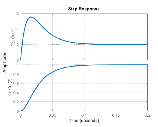
A plot of the motor response with feedforward compensation is shown in Fig. 9.2.1. As expected, the motor speed asymptotically approaches unity in the steady-state.

Figure \(\PageIndex{1}\): The step response of the DC motor with pole placement controller and feedforward compensation: armature current (top); motor speed (bottom).

Example \(\PageIndex{2}\)

The state variable model of a mass–spring–damper is given as: \[\frac{\rm d}{\rm dt} \left[\begin{array}{c} {x} \\ {v} \end{array}\right]=\left[\begin{array}{cc} {0} & {1} \\ {-10} & {-1} \end{array}\right]\left[\begin{array}{c} {x} \\ {v} \end{array}\right]+\left[\begin{array}{c} {0} \\ {1} \end{array}\right]f, \;\;x=\left[\begin{array}{cc} {1} & {0} \end{array}\right]\left[\begin{array}{c} {x} \\ {v} \end{array}\right] \nonumber \]

A pole placement controller for the model was previously designed as: \(f=-3v\).

The control law is modified to include a feedforward gain as: \(f=-3v+k_{r} r.\)

The closed-loop system model is given as: \(\frac{\rm d}{\rm dt} \left[\begin{array}{c} {x} \\ {v} \end{array}\right]=\left[\begin{array}{cc} {0} & {1} \\ {-10} & {-4} \end{array}\right]\left[\begin{array}{c} {x} \\ {v} \end{array}\right]+k_{r} r\).

The steady-state output is: \(y_{ss} =0.1k_{r} r_{ss}\). Hence, we may choose \(k_{r} =10\) for error-free tracking. The resulting control law is given as: \(f=-3v+10\, r.\)