1.7: Physical Estimates

Your gut understands not only the social world but also the physical world. If you trust its feelings, you can tap this vast reservoir of knowledge. For practice, we’ll estimate the salinity of seawater(Section 1.7.1), human power output (Section 1.7.2), and the heat of vaporization of water (Section 1.7.3).

1.7.1 Salinity of seawater

To estimate the salinity of seawater, which will later help you estimate the conductivity of seawater(Problem 8.10), do not ask your gut directly: “How do you feel about, say, 200 millimolar?” Although that kind of question worked for estimating population density (Section 1.6), here, unless you are a chemist, the answer will be: “I have no clue. What is a millimolar anyway? I have almost no experience of that unit.” Instead, offer your gut concrete data—for example, from a home experiment: adding salt to a cup of water until the mixture tastes as salty as the ocean.

This experiment can be a thought or a real experiment—another example of using multiple methods (Section 1.5). As a thought experiment, I ask my gut about various amounts of salt in a cup of water. When I propose adding 2 teaspoons, it responds, “Disgustingly salty!” At the lower end, when I propose adding 0.5 teaspoons, it responds, “Not very salty.” I’ll use 0.5 and 2 teaspoons as the lower and upper endpoints of the range. Their midpoint, the estimate from the thought experiment, is 1 teaspoon per cup.

I tested this prediction at the kitchen sink. With 1 teaspoon (5 milliliters) of salt, the cup of water indeed had the sharp, metallic taste of seawater that I have gulped after being knocked over by large waves. A cup of water is roughly one-fourth of a liter or 250 cubic centimeters. By mass, the resulting salt concentration is the following product:

\[\frac{\cancel{1 tsp \: salt}}{\cancel{1 cup \: water}} \times \frac{\cancel{1 cup \: water}}{250g \: water} \times \frac{\cancel{5 cm^{3} \: salt}}{\cancel{1 tsp \: salt}} \times \frac{2g \: salt}{\cancel{1 cm^{3} \: salt}}\]

The density of 2 grams per cubic centimeter comes from my gut feeling that salt is a light rock, so it should be somewhat denser than water at 1 gram per cubic centimeter, but not too much denser. (For an alternative method, more accurate but more elaborate, try Problem 1.10.) Then doing the arithmetic gives a 4 percent salt-to-water ratio (by mass).

The actual salinity of the Earth’s oceans is about 3.5 percent—very close to the estimate of 4 percent. The estimate is close despite the large number of assumptions and approximations—the errors have mostly canceled. Its accuracy should give you courage to perform home experiments whenever you need data for divide-and-conquer estimates.

Exercise \(\PageIndex{1}\): Density of water

Estimate the density of water by asking your gut to estimate the mass of water in a cup measure (roughly one-quarter of a liter).

Exercise \(\PageIndex{2}\): Density of salt

Estimate the density of salt using the volume and mass of a typical salt container that you find in a grocery store. This value should be more accurate than my gut estimate in Section 1.7.1 (which was 2 grams per cubic centimeter).

1.7.2 Human power output

Our second example of talking to your gut is an estimate of human power output—a power that is useful in many estimates (for example, Problem 1.17). Energies and powers are good candidates for divide-and-conquer estimates, because they are connected by the subdivision shown in the following equation and represented in the tree in the margin:

\[power = \frac{energy}{time}\]

In particular, let’s estimate the power that a trained athlete can generate for an extended time (not just during a few-seconds-long, high-power burst). As a proxy for that power, I’ll use my own burst power output with two adjustment factors:

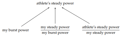
Maintaining a power is harder than producing a quick burst. Therefore, the first adjustment factor, my steady power divided by my burst power, is somewhat smaller than 1—maybe 1/2 or 1/3. In contrast, an athlete’s power output will be higher than mine, perhaps by a factor of 2 or 3: Even though I am sometimes known as the street-fighting mathematician [33], I am no athlete. Then the two adjustment factors roughly cancel, so my burst power should be comparable to an athlete’s steady power.

To estimate my burst power, I performed a home experiment of running up a flight of stairs as quickly as possible. Determining the power output requires estimating an energy and a time:

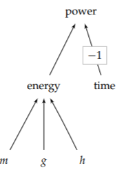
\[\textrm{energy} = \underbrace{\textrm{mass}}_{m} \times \underbrace{\textrm{gravity}}_{g} \times \underbrace{\textrm{height}}_{h}.\]

In the academic building at my university, a building with high ceilings and staircases, I bounded up a staircase three stairs at a time. The staircase was about 12 feet or 3.5 meters high. Therefore, my mechanical energy output was roughly 2000 joules:

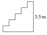
\[E \sim 65 kg \times 10 m s^{-2} \times 3.5 m \sim 2000J \]

(The units are fine: 1 J = 1 kg m² s⁻2.)

The remaining leaf is the time: how long the climb took me. I made it in 6 seconds. In contrast, several students made it in 3.9 seconds—the power of youth! My mechanical power output was about 2000 joules per 6 seconds, or about 300 watts. (To check whether the estimate is reasonable, try Problem 1.12, where you estimate the typical human basal metabolism.)

This burst power output should be close to the sustained power output of a trained athlete. And it is. As an example, in the Alpe d’Huez climb in the 1989 Tour de France, the winner—Greg LeMond, a world-class athlete—put out 394 watts (over a 42.5-minute period). The cyclist Lance Armstrong, during the time-trial stage during the Tour de France in 2004, generated even more: 495 watts (roughly 7 watts per kilogram). However, he publicly admitted to blood doping to enhance performance. Indeed, because of widespread doping, many cycling power outputs of the 1990s and 2000s are suspect; 400 watts stands as a legitimate world-class sustained power output.

Exercise \(\PageIndex{3}\): Energy in a 9-volt battery

Estimate the energy in a 9-volt battery. Is it enough to launch the battery into orbit?

Exercise \(\PageIndex{4}\): Basal metabolism

Based on our daily caloric consumption, estimate the human basal metabolism.

Exercise \(\PageIndex{5}\): Energy measured in person flights of stairs

How many flights of stairs can you climb using the energy in a stick (100 grams) of butter?

1.7.3 Heat of vaporization of water

Our final physical estimate concerns the most important liquid on Earth.

What is the heat of vaporization of water?

Because water covers so much of the Earth and is such an important part of the atmosphere (clouds!), its heat of vaporization strongly affects our climate—whether through rainfall (Section 3.4.3) or air temperatures.

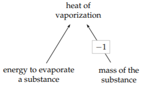
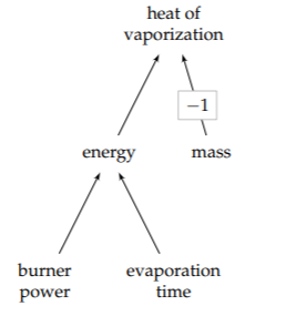
Heat of vaporization is defined as a ratio:

\[\frac{\textrm{energy to evaporate a substance}}{\textrm{amount of the substance}}.\]

where the amount of substance can be measured in moles, by volume, or(most commonly) by mass. The definition provides the structure of the tree and of the estimate based on divide-and-conquer reasoning.

For the mass of the substance, choose an amount of water that is easy to imagine—ideally, an amount familiar from everyday life. Then your gut can help you make estimates. Because I often boil a few cups of water at a time, and each cup is few hundred milliliters, I’ll imagine 1 liter or 1 kilogram of water.

The other leaf, the required energy, requires more thought. There is a common confusion about this energy that is worth discussing.

Is it the energy required to bring the water to a boil?

No: The energy has nothing to do with the energy required to bring the water to a boil! That energy is related to water’s specific heat c_p. The heat of vaporization depends on the energy needed to evaporate—boil away—the water, once it is boiling. (You compare these energies in Problem 5.61.)

Energy subdivides into power times time (as when we estimated human power output in Section 1.7.2). Here, the power could be the power output of one burner; the time is the time to boil away the liter of water. To estimate these leaves, let’s hold a gut conference.

For the time, my dialogue is as follows.

LB: How does 1 minute sound as a lower bound?

RB: Way too short—you’ve left boiling water on the stove unattended for longer without its boiling away!

LB: How about 3 minutes?

RB: That’s on the low side. Maybe that’s the lower bound.

LB: Okay. For the upper bound, how about 100 minutes?

RB: That time feels way too long. Haven’t we boiled away pots of water in far less time?

LB: What about 30 minutes?

RB: That’s long, but I wouldn’t be shocked, only fairly surprised, if it took that long. It feels like the upper bound.

My range is therefore 3…30 minutes. Its midpoint—the geometric mean of the endpoints—is about 10 minutes or 600 seconds.

For variety, let’s directly estimate the burner power, without estimating lower and upper bounds.

LB: How does 100 watts feel?

RB: Way too low: That’s a lightbulb! If a lightbulb could boil away water so quickly, our energy troubles would be solved.

LB (feeling chastened): How about 1000 watts (1 kilowatt)?

RB: That’s a bit low. A small appliance, such as a clothes iron, is already 1 kilowatt.

LB (raising the guess more slowly): What about 3 kilowatts?

RB: That burner power feels plausible.

Let’s check this power estimate by subdividing power into two factors, voltage and current:

\[power = voltage \times current\]

An electric stove requires a line voltage of 220 volts, even in the United States where most other appliances require only 110 volts. A standard fuse is about 15 amperes, which gives us an idea of a large current. If a burner corresponds to a standard fuse, a burner supplies roughly 3 kilowatts:

\[200V \times 15A \approx 3000W\]

This estimate agrees with the gut estimate, so both methods gain plausibility—which should give you confidence to use both methods for your own estimates. As a check, I looked at the circuit breaker connected to my range, and it is rated for 50 amperes. The range has four burners and an oven, so 15 amperes for one burner (at least, for the large burner) is plausible.

We now have values for all the leaf nodes. Propagating the values toward the root gives the heat of vaporization (L_vap) as roughly 2 megajoules per kilogram:

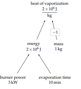
\[L_{vap} \sim \frac{\overbrace{3kW}^{\textrm{power}} \times \overbrace{600s}^{\textrm{time}}}{\underbrace{1 \: kg}_{\textrm{mass}}} \approx 2 \times 10^{6} \textrm{J kg}^{-1}.\]

The true value is about 2.2×10⁶ joules per kilogram. This value is one of the highest heats of vaporization of any liquid. As water evaporates, it carries away significant amounts of energy, making it an excellent coolant (Problem 1.17).