3.1: Invariants

We use symmetry and conservation whenever we find a quantity that, despite the surrounding complexity, does not change. This conserved quantity is called an invariant. Finding invariants simplifies many problems.

Our first invariant appeared unannounced in Section 1.2 when we estimated the carrying capacity of a lane of highway. The carrying capacity—the rate at which cars flow down the lane—depends on the separation between the cars and on their speed. We could have tried to estimate each quantity and then the carrying capacity. However, the separation between cars and the cars’ speeds vary greatly, so these estimates are hard to make reliably.

Instead, we invoked the 2-second following rule. As long as drivers obey it, the separation between cars equals 2 seconds of driving. Therefore, one car flows by every 2 seconds—which is the lane’s carrying capacity (in cars per time). By finding an invariant, we simplified a complex, changing process. When there is change, look for what does not change! (This wisdom is from Arthur Engel’s Problem-Solving Strategies [12].)

3.1.1 To run or walk in the rain?

We’ll practice with this tool by deciding whether to run or walk in the rain. It’s pouring, your umbrella is sitting at home, and home lies a few hundred meters away.

To minimize how wet you become, should you run or walk?

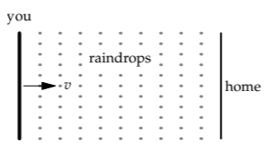
Let's answer this question with three simplifications. First, assume that there is no wind, so the rain is falling vertically. Second, assume that the rain is steady. Third, assume that you are a thin sheet: You have zero thickness along the direction toward your house (this approximation was more valid in my youth). Equivalently, your head is protected by a water-proof cap, so you do not care whether raindrops hit your head. You try to minimize just the amount of water hitting your front.

Your only degree of freedom—the only parameter that you get to choose—is your speed. A high speed leaves you in the rain for less time. However, it also makes the rain come at you more directly (more horizontally). But what remains constant, independent of your speed, is the volume of air that you sweep out. Because the rain is steady, that volume contains a fixed number of raindrops, independent of your speed. Only these raindrops hit your front. Therefore, you get equally wet, no matter your speed.

This surprising conclusion is another application of the principle that when there is change, look for what does not change. Here, we could change our speed by choosing to walk or run. Yet no matter what our speed, we sweep out the same volume of air—our invariant.

Because the conclusion of this invariance analysis, that it makes no difference whether you walk or run, is surprising, you might still harbor a nagging doubt. Surely running in the rain, which we do almost as a reflex, provide some advantage over a leisurely stroll.

Is it irrational to run to avoid getting wet?

If you are infinitely thin, and are just a rectangle moving in the rain, then the preceding analysis applies: Whether you run or walk, your front will absorb the same number of raindrops. But most of us have a thickness, and the number of drops landing on our head depends on our speed. If your head is exposed and you care how many drops land on your head, then you should run. But if your head is covered, feel free to save your energy and enjoy the stroll. Running won’t keep you any dryer.

3.1.2 Tiling a mouse-eaten chessboard

Often a good way to practice a new tool is on a mathematical problem. Then we do not add the complexity of the physical world to the problem of learning a new tool. Here, therefore, is a mathematical problem: a solitaire game.

A mouse comes and eats two diagonally opposite corners out of a standard, 8 × 8 chessboard. We have a box of rectangular, 2 × 1 dominoes.

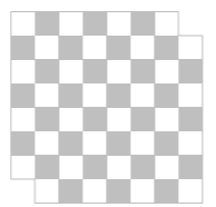
Can these dominoes tile the mouse-eaten chessboard? In other words, can we lay down the dominoes to cover every square exactly once (with no empty squares and no overlapping dominoes)?

Placing a domino on the board is one move in this solitaire game. For each move, you choose where to place the domino—so you have many choices at each move. The number of possible move sequences grows rapidly. Instead of examining all these sequences, we’ll look for an invariant: a quantity unchanged by any move of the game.

Because each domino covers one white square and one black square, the following quantity I is invariant (remains fixed):

\[I = \textrm{uncovered black squares} - \textrm{uncovered white squares}\]

On a regular chess board, with 32 white squares and 32 black squares, the initial position has I = 0. The nibbled board has two fewer black squares, so I starts at 30 − 32 = −2. In the winning position, all squares are covered, so I = 0. Because I is invariant, we cannot win: The dominoes cannot tile the nibbled board.

Each move in this game changes the chessboard. By finding what does not change, an invariant, we simplified the analysis.

Invariants are powerful partly because they are abstractions. The details of the empty squares—their exact locations—lie below the abstraction barrier. Above the barrier, we see only the excess of black over white squares. The abstraction contains all the information we need in order to know that we can never tile the chessboard.

Exercise \(\PageIndex{1}\): Cube Solitaire

A cube has numbers at each vertex; all vertices start at 0 except for the lower left corner, which starts at 1. The moves are all of the same form: Pick any edge and increment its two vertices by one. The goal of this solitaire game is to make all vertices multiples of 3.

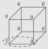
For example, picking the bottom edge of the front face and then the bottom edge of the back face, makes the following sequence of cube configurations:

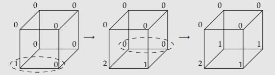
Although no configuration above wins the game, can you win with a different move sequence? If you can win, give a winning sequence. If you cannot win, prove that you cannot.

Hint: Create analogous but simpler versions of this game.

Exercise \(\PageIndex{2}\): Triplet solitaire

Here is another solitaire game. Start with the triplet (3, 4, 5). At each move, choose any two of the three numbers. Call the choices a and b. Then make the following replacements:

\(a \rightarrow 0.8a - 0.6b\);

\(b \rightarrow 0.6a + 0.8b\).

Can you reach (4, 4, 4)? If you can, give a move sequence; otherwise, prove that it is impossible.

Exercise \(\PageIndex{3}\): Triplet-solitaire moves as rotations in space

At each step in triplet solitaire (Problem \(\PageIndex{2}\)), there are three possible moves, depending on which pair of numbers from among a, b, and c you choose to replace. Describe each of the three moves as a rotation in space. That is, for each move, give the rotation axis and the angle of rotation.

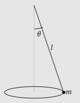
Exercise \(\PageIndex{4}\): Conical pendulum

Finding the period of a pendulum, even at small amplitudes, requires calculus because of the pendulum’s varying speed. When there is change, look for what does not change. Accordingly, Christiaan Huygens (1629–1695), called “the most ingenious watchmaker of all time” [20, p. 79] by the great physicist Arnold Sommerfeld, analyzed the motion of a pendulum moving in a horizontal circle (a conical pendulum). Projecting its two-dimensional motion onto a vertical screen produces one-dimensional pendulum motion; thus, the period of the two-dimensional motion is the same as the period of one-dimensional pendulum motion! Use that idea to find the period of a pendulum (without calculus!).

3.1.3 Logarithmic scales

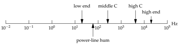
In the solitaire game in Section 3.1.2, a move covered two chessboard squares with a domino. In the game of understanding the world, a frequent move is changing the system of units. As in solitaire, ask, "When such a move is made, what is invariant?" As an example to crystallize our thinking, here are frequencies related to human hearing. Let's graph them using kilohertz (kHz) as the unit. The frequencies then arrange themselves as follows:

low end of hearing: 20 Hz

piano middle C: 262 Hz

highest piano C: 4186 Hz

high end of hearing: 20 kHz

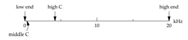
Now let’s change units from kilohertz to hertz (Hz)—and keep the 0, 10, and 20 labels at their current positions on the page. This change magnifies every spacing by a factor of 1000: The new 20 hertz is where 20 kilohertz was (about 4 inches or 10 centimeters to the right of the origin), and 20 kilohertz, the high end of human hearing, sits 100 meters to ourright—far beyond the borders of the page. This new scale is not very useful.

However, we missed the chance to use an invariant: the ratio between frequencies. For example, the ratio between the upper end of human hearing (20 kilohertz) and middle C (262 hertz) is roughly 80. If we use a representation based on ratio rather than absolute difference, then the spacing between frequencies would not change even when we changed the unit.

We have such a representation: logarithms! On a logarithmic scale, a distance corresponds to a ratio rather than a difference. To see the contrast, let’s place the numbers from 1 to 10 on a logarithmic scale.

The physical gap between 1 and 2 represents not their difference but rather their ratio, namely 2. According to my ruler, the gap is approximately 3.16 centimeters. Similarly, the physical gap between 2 and 3—approximately 1.85 centimeters—represents the smaller ratio 1.5. In contrast to their relative positions on a linear scale, 2 and 3 on a logarithmic scale are closerthan 1 and 2 are. On a logarithmic scale, 1 and 2 have the same separation as 2 and 4: Both gaps represent a ratio of 2 and therefore have the same physical size (3.16 centimeters).

Exercise \(\PageIndex{5}\): Practice with ratio thinking

On a logarithmic scale, how does the physical gap between 2 and 8 compare to the gap between 1 and 2? Decide based on your understanding of ratios; then check your reasoning by measuring both gaps.

Exercise \(\PageIndex{6}\): More practice with ratio thinking

Is the gap between 1 and 10 less than twice, equal to twice, or more than twice the gap between 1 and 3? Decide based on your understanding of ratios; then check your reasoning by measuring both gaps.

Exercise \(\PageIndex{7}\): Moving along a logarithmic scale

On the logarithmic scale in the text, the gap between 2 and 3 is approximately 1.85 centimeters. Where do you land if you start at 6 and move 1.85 centimeters rightward? Decide based on your understanding of ratios; then check your reasoning by using a ruler to find the new location.

Exercise \(\PageIndex{8}\): Extending the scale to the right

On the logarithmic scale in the text, the gap between 1 and 10 is approximately 10.5 centimeters. If the scale were extended to include numbers up to 1000, how large would the gap between 10 and 1000 be?

Exercise \(\PageIndex{9}\): Extending the scale to the left

If the logarithmic scale were extended to include numbers down to 0.01, how far to the left of 1 would you have to place 0.04?

On a logarithmic scale, the frequencies related to hearing arrange themselves as follows:

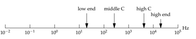
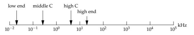
Changing the units to kilohertz just shifts all the frequencies, but leaves their relative positions invariant:

Exercise \(\PageIndex{10}\): Acoustic energy fluxes

In acoustics, sound intensity is measured by energy flux, which is measured in decibels (dB)—a logarithmic representation of watts per square meter. On the decibel scale, 0 decibels corresponds to the reference level of 10⁻¹² watts per square meter. Every 10 decibels (or 1 bel) represents an increase in energy flux of a factor of 10 (thus, 20 decibels represents a factor-of-100 increase in energy flux).

a. How many watts per square meter is 60 decibels (the sound level of normal conversation)?

b. Place the following energy fluxes on a decibel scale: 10−9 watts per square meter (an empty church), 10−2 watts per square meter (front row at an orchestra concert), and 1 watt per square meter (painfully loud).

Logarithmic scales offer two benefits. First, as we saw explicitly, logarithmic scales incorporate invariance. The second benefit was only implicit in the previous discussion: Logarithmic scales, unlike linear scales, allow us to represent a huge range. For example, if we include power-line hum (50 or 60 hertz) on the linear frequency scale on p. 61, we can hardly distinguish its position from 0 kilohertz. The logarithmic scale has no problem.

In our fallen world, benefits usually conflict. One usually has to sacrifice one benefit for another (speed for accuracy or justice for mercy). With logarithmic scales, however, we can eat our cake and have it.

Exercise \(\PageIndex{11}\)

Labeling a logarithmic scale

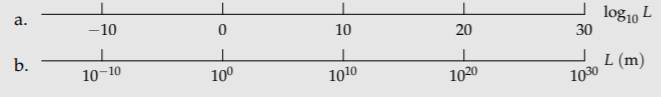
Let’s make a scale to represent sizes in the universe, from protons (10−15 meters) to galaxies (1030 meters), with people and bacteria in between. With such a large range, we should use a logarithmic scale for size L. Which one of these two ways of labeling the scale is correct, and which way is nonsense?

Logarithmic scales can make otherwise obscure symbolic calculations intuitive. An example is the geometric mean, which we used in Section 1.6 to make gut estimates:

\[estimate = \sqrt{lower \: bound \times upper \: bound}\]

Geometric means also occur in the physical world. As you found in Problem 2.9, the distance d to the horizon, as seen from a height h above the Earth's surface, is

\[d \approx \sqrt{hD}\]

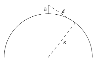
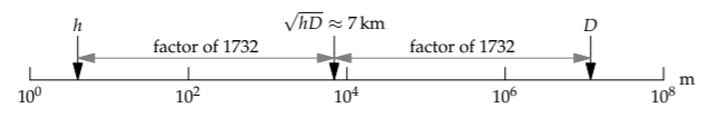
where \(D = 2R_{Earth}\) is the diameter of the Earth. Imagine a lifeguard sitting with his or her eyes at a height h= 4 meters above sea level. Then the distance to the horizon is

\[d \approx (\underbrace{4m}_{h} \times \underbrace{120000 km}_{D})^{1/2}.\]

To do the calculation, we convert 12,000 kilometers to 1.2 × 10⁷ meters, calculate 4 × 1.2×10⁷, and compute the square root:

\[d \approx \sqrt{4 \times 1.2 \times 10^{7}} m \approx 7000m = 7km\]

In this symbolic form with a square root, the calculation obscures the fundamental structure of the geometric mean. We first calculate hD, which is an area (and often contains, as it did here, a huge number). Then we take the square root to get back a distance. However, the area has nothing to do with the structure of the problem. It is merely a bookkeeping device.

Bookkeeping devices are useful; they are how you tell a computer what to calculate. However, to understand the calculation, we, as humans, should use a logarithmic scale to represent the distances. This scale captures the structure of the problem.

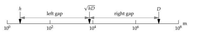
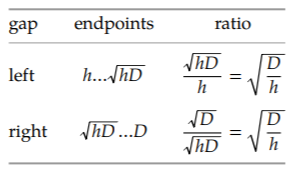
How can we describe the position of the geometric mean \(\sqrt{hD}\)?

The first clue is that the geometric mean, because it is a mean, because it is a mean, lies somewhere between h and D. This property is not obvious from the calculation using the square root. To find where the geometric mean lies, mind the gaps. On a logarithmic scale, a gap represents the ratio of its endpoints. As shown in the table, the left and right gaps. On a logarithmic scale, a gap represents the ratio of its endpoints. As shown in the table, the left and right gaps represent the same ratio, namely \(\sqrt{D/h}\)! Therefore, on the logarithmic scale, the geometric mean lies exactly halfway between h and D.

Based on this ratio representation, we can rephrase the geometric-mean calculation in a form that we can do mentally

What distance is as large compared to 4 meters as 12,000 kilometers is compared to it?

For lack of imagination, my first guess is 1 kilometer. It’s 12,000 times smaller than the diameter D (which is 12,000 kilometers), but only 250 times larger than the height h (4 meters). My guess of 1 kilometer is therefore somewhat too small.

How is a guess of 10 kilometers?

It’s 2500 times larger than h, but only 1200 times smaller than D. I overshot slightly. How about 7 kilometers? It’s roughly 1750 times larger than 4 meters, and roughly 1700 times smaller than 12 000 kilometers. Those gaps are close to each other, so 7 kilometers is the approximate geometric mean.

Similarly, when we make gut estimates, we should place our lower and upper estimates on a logarithmic scale. Our best gut estimate is then their midpoint. What a simple picture!

Should all quantities be placed on a logarithmic scale?

No. An illustrative contrast is between size and position. Both quantities have the same units. But size ranges from 0 to ∞, whereas position ranges from −∞ to ∞. Position therefore cannot be placed on a logarithmic scale (where would you put −1 meter?). In contrast, size (a magnitude) belongs on a logarithmic scale. In general, location parameters, such as position, should not be placed on a logarithmic scale but magnitudes should.