4.2: Finding Scaling Exponents

The dinner example (Section 4.1) used linear proportionality: When the number of dinner guests doubled, so did the amount of food. The relation between the quantities had the form \( y \alpha x\) or, more explicitly, \(y \alpha x^{1}\). The exponent, which here is 1, is called the scaling exponent. For that reason, proportionalities are often called scaling relations. Scaling exponents are a powerful abstraction: Once you know the scaling exponent, you usually do not care about the mechanism underlying it.

4.2.1 Warmup

After linear proportionality, the next simplest and most common type of proportionality is quadratic--a scaling exponent of 2--and its close cousin, a scaling exponent of 1/2. As an example, here is a big circle with diameter \(d_{big} = \sqrt{5} cm.\)

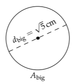
What is the diameter of the circle with one-half the area of this circle?

Let’s first do the very common brute-force solution, which does not use proportional reasoning, so that you see what not to do. It begins with the area of the big circle:

\[A_{big} = \frac{\pi}{4} d^{2}_{big} = \frac{5}{4} \pi cm^{2}.\]

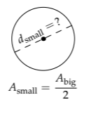
The area of the small circle A_small is A_big/2, so A_small = \(5 \pi / 8 cm^{2}\) Therefore, the diameter of the small circle is given by

\[d_{small} \sqrt{\frac{A_{small}}{\pi/4}} = \sqrt{\frac{5}{2}} cm.\]

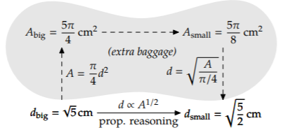
Although this result is correct, by including \(\pi/4\) and then dividing it out, we run around Robin Hood’s barn (all of Sherwood forest) to reach a simple result. There must be a more elegant and insightful approach.

This improved approach also starts with the relation between a circle’s area and its diameter: \(A = \pi d^{2}/4\). However, it discards the complexity early—in the next step—rather than carrying it through the analysis and having it vanish only at the end. An everyday analog of this approach is packing for a trip. Rather than dragging around books that you will not read or clothes that you will not wear, prune early and travel light: Pack only what you will use and set aside the rest.

To lighten your problem-solving luggage, observe that all circles, independent of their diameter, have the same prefactor \(\pi /4\) connecting d² and A. Therefore, when we make a proportionality or scaling relation between A and d, we discard the prefactor. The result is the following quadratic proportionality (one where the scaling exponent is 2):

\[A \alpha d^{2}\]

For finding the new diameter, we need the inverse scaling relation:

\[d \alpha A^{1/2}\]

In this form, the scaling exponent is 1/2. This proportionality is shorthand for the ratio relation

\[\frac{d_{small}}{d_{big}} = (\frac{A_{small}}{A_{big}})^{1/2}.\]

The area ratio is 1/2, so the diameter ratio is \(1/ \sqrt{2}\) Because the large diameter is \(\sqrt{5}\) cm, the small diameter is \(\sqrt{5/2}\) cm.

The proportional-reasoning solution is shorter than the brute-force approach, so it offers fewer places to go wrong. It is also more general: It shows that the result does not require that the shape be a circle. As long as the area of the shape is proportional to the square of its size (as a length)—a relation that holds for all planar shapes—the length ratio is \(1/ \sqrt{2}\) whenever the area ratio is 1/2. All that matters is the scaling exponent.

Exercise \(\PageIndex{1}\): Length of the horizontal bisecting path

In Problem 3.23, about the shortest path that bisects an equilateral triangle, one candidate path is a horizontal line. How long is that line relative to a side of the triangle?

Areas are connected to flux, because flux is rate per area. Thus, the scaling exponent for area—namely, 2—appears in flux relationships. For example:

What is the solar flux at Pluto’s orbit?

The solar flux F at a distance r from the Sun is the solar luminosity L_Sun—the radiant power output of the sun—spread over a sphere with radius r:

\[F = \frac{L_{Sun}}{4 \pi r^{2}}.\]

Even as r changes, the solar luminosity remains the same (conservation!), as does the factor 4 \(\pi\). Therefore, in the spirit of packing light for a trip, simplify the equality \(F=L_{Sun}/4 \pi r^{2}\) to the proportionality.

\[F \alpha r^{-2}\]

by discarding the factors L_Sun and \(4 \pi\). The scaling exponent here is −2: The minus sign indicates the inverse proportionality between flux and area, and the 2 is the scaling exponent connecting r to area.

The scaling relation is shorthand for

\[\frac{F_{\textrm{Pluto's orbit}}}{F_{\textrm{Earth's orbit}}} =(\frac{r_{\textrm{Pluto's orbit}}}{r_{\textrm{Earth's orbit}}})^{-2},\]

or

\[F_{\textrm{Pluto's orbit}} = F_{\textrm{Earth's orbit}} (\frac{r_{\textrm{Pluto's orbit}}}{r_{\textrm{Earth's orbit}}})^{-2}.\]

The ratio of orbital radii is roughly 40. Therefore, the solar flux at Pluto’s orbit is roughly 40^-2 or 1/1600 of the flux at the Earth’s orbit. The resulting flux is roughly 0.8 watts per square meter:

\[F_{\textrm{Pluto's orbit}} = \frac{1300W}{m^{2}} \times \frac{1}{1600} \approx \frac{0.8W}{m^{2}}\]

Receiving such a small amount of sunlight, Pluto must be very cold. We can estimate its surface temperature with a further proportionality.

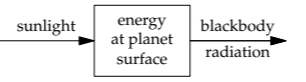
Surface temperature depends mostly on so-called blackbody radiation. The surface temperature is the temperature at which the radiated flux equals the incoming flux; we are making another box model. The radiated flux is given by the blackbody formula (which we will derive in Section 5.5.2)

\[F= \sigma T^{4}\]

where T is the temperature, and \(\sigma\) is the Stefan-Boltzmann constant:

\[\sigma \approx 5.7 \times 10^{-8} \frac{W}{m^{2}K^{4}}.\]

What is the resulting surface temperature on Pluto?

As with any proportional-reasoning calculation, there is a long-winded, brute-force alternative (try Problem 4.5). The elegant approach directly uses the proportionalities.

\[T \: \propto \: F^{1/4} \: and \: F \: \propto \: r^{-2},\]

where r is the orbital radius. Together, they produce a new proportionality

\[T \: \propto (r^{-2})^{1/4} = r^{-1/2}.\]

A compact graphical notation, similar to the divide-and-conquer trees, encapsulates this derivation:

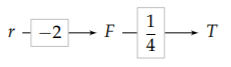
As indicated by the \(r \rightarrow F\) arrow, changing r changes F. The boxed number along the arrow gives the scaling exponent. Therefore, the \(r \rightarrow F\) arrow represents \(F \: \propto \: r^{-2}\). The \(F \rightarrow T\) arrow indicates that changing F changes T and, in particular, that \(T \: \propto \: F^{1/4}\).

To find the scaling exponent connecting r to T, multiply the scaling exponents along the path:

\[-2 \times \frac{1}{4} = -\frac{1}{2}\]

Exercise \(\PageIndex{2}\): Explaining the graphical notation

In our graphical representation of scaling relations, why is the final scaling exponent the product, rather than the sum, of the scaling exponents along the way?

This scaling exponent represents the following comparison:

\[\frac{T_{\textrm{Earth}}}{T_{\textrm{Pluto}}} = (\frac{r_{\textrm{Earth's orbit}}}{r_{\textrm{Pluto's orbit}}})^{-1/2} = (\frac{r_{\textrm{Pluto's orbit}}}{r_{\textrm{Earth's orbit}}})^{1/2}\]

(The rightmost form, with the positive exponent, is more direct than the intermediate form, because it does not first produce a fraction smaller than 1 and then take its reciprocal with a negative exponent.) The ratio of orbital radii is 40, so the ratio of surface temperatures should be \(\sqrt{40}\) or roughly 6. Pluto's surface temperature should be roughly 50K:

\[T_{\textrm{Pluto}} \approx \frac{T_{\textrm{Earth}}}{6} \approx \frac{293K}{6} \approx 50K\]

Pluto’s actual mean surface temperature is 44 K, very close to our prediction based on proportional reasoning.

Exercise \(\PageIndex{3}\): Explaining the discrepancy

Why is our prediction for Pluto’s mean temperature slightly too high?

Exercise \(\PageIndex{4}\): Brute-force calculation of surface temperature

To practice recognizing common but inferior problem-solving methods, use the brute-force method to estimate the surface temperature on Pluto: (a) From the solar flux at Pluto’s orbit, calculate the solar flux averaged over the surface; (b) use that flux to estimate a blackbody temperature.

4.2.2 Orbital periods

In the preceding examples, the scaling relations formed chains (trees without branching):

food for a dinner party: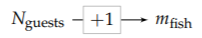

area of a circle: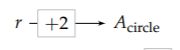

surface temperature :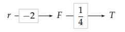

More elaborate relationships also occur—as we will find in rederiving a famous law of planetary motion.

How does a planet’s orbital period depend on its orbital radius r?

We’ll study the special case of circular orbits (many planetary orbits are close to circular). Our exploratory thinking is often aided by making proportionality questions concrete. Therefore, rather than finding the scaling exponent using the abstract notion of “depend on,” answer the doubling question: “When I double this quantity, what happens to that quantity?”

What is so special about doubling?

Doubling—multiplying by a factor of 2—is the simplest useful change. A factor of 1 is simpler; however, being no change at all, it is too simple.

What happens to the period if we double the orbital radius?

The most direct effect of doubling the orbital radius is that gravity gets weaker. Because the gravitational force is an inverse-square force--that is, \(F \: \alpha \: r^{-2}\) --the gravitational force falls by a factor of 4. A compact and intuitive notation for these changes is to mark the change directly under the quantity: A notation of \(\times n\) indicates multiplication by a factor of n.

\[\underbrace{F}_{\times \frac{1}{4}} \propto \underbrace{r}_{\times 2} ^{-2}.\]

Because force is proportional to acceleration, the planet’s acceleration a falls by the same factor of 4.

In circular motion, acceleration and velocity are related by \(a = \frac{v^{2}}{r}\). (We will derive this relation in Section 5.1.1 and Section 6.3.4, with two different reasoning tools.) Therefore, the orbital velocity v is \(\sqrt{ar}\), and doubling the radius increases the orbital speed by a factor of \(\sqrt{1/2}\):

\[\underbrace{v}_{\times \sqrt{\frac{1}{2}}} = (\underbrace{a}_{\times{\frac{1}{4}}} \times \underbrace{r}_{\times 2})^{1/2}.\]

Although this calculation is correct, when it is states as a factor of \(\sqrt{1/2}\) it confounds our expectations and produces numerical whiplash. As we finish reading "increases by a factor of," we expect a number greater than 1. But we get a number smaller than 1. An increase by a factor smaller than 1 is more simply described as a decrease. Therefore, it is more direct to say that the orbital speed falls by a factor of \(\sqrt{2}\).

The orbital period is \(T \sim r/v\) (the ~ contains the dimensionless prefactor 2 \(\pi\)), so it increases by a factor of 2^3/2 :

\[\underbrace{T}_{\times 2^{3/2}} \sim \underbrace{r}_{\times 2} \times \underbrace{v^{-1}}_{\times \sqrt{2}} .\]

In summary, doubling the orbital radius multiplies the orbital period by 2^3/2. In general, the connection between r and T is

\[T \: \propto \: r^{3/2}.\]

This result is Kepler's third law for circular orbits. Our scaling analysis has the following graphical representation:

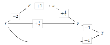
In this structure, the new feature is that two paths reach the orbital velocity v. There we add the incoming exponents.

1. 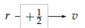represents the \(\sqrt{r}\) in \(v= \sqrt{ar}\). It carries +1/2 powers of r.

2. 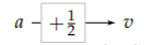represents the \(\sqrt{a}\) in \(v= \sqrt{ar}\). To determine how many powers of r flow through this arrow, follow the chain containing it:

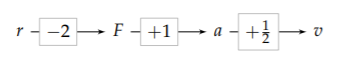
One power of r starts at the left side. It becomes −2 powers after passing through the first scaling exponent and arriving at F. It remains −2 powers on arrival at a. Finally, it becomes −1 power on arrival at v. This path therefore carries −1 power of r.

Its contribution is the result of multiplying the three scaling exponents along the chain:

\[\underbrace{-2}_{r \rightarrow F} \times \underbrace{+1}_{F \rightarrow a} \times \underbrace{- \frac{1}{2}}_{a \rightarrow v} = -1.\]

The -1 power carried by the three-link chain, representing r^-1 , combines with the +1/2 from the direct \(r \rightarrow v\), which represents r^+1/2 . Adding the exponents or r, the result is that v contains -1/2 powers of r.

\[v \propto \underbrace{r^{-1}}_{\textrm{via} F} \times \underbrace{r^{+1/2}}_{\textrm{direct}} = r^{-1/2}.\]

Let's practice the same reasoning by finding the scaling relation connecting T and r--which is Kepler's third law. The direct \(r \rightarrow T\) arrow, with a scaling exponent of +1, carries +1 powers of r. The \(v \rightarrow T\) arrow carries +1/2 powers of r:

\[v \propto \underbrace{r^{-1}}_{\textrm{via } F} \times \underbrace{r^{+1/2}}_{\textrm{direct}} = r^{1/2}.\]

Together, the two arrows contribute +3/2 powers of r and give us Kepler’s third law:

\[\underbrace{-\frac{1}{2}}{r \rightarrow v} \times \underbrace{-1}{v \rightarrow T} = + \frac{1}{2}.\]

To summarize the exponent rules, for which we now have several illustrations: (1) Multiply exponents along a path, and (2) add exponents when paths meet.

Now let’s apply Kepler’s third law to a nearby planet.

How long is the Martian year?

The proportionality \(T \: \propto \: r^{3/2}\) is shorthand for the comparison

\[\frac{T_{Mars}}{T_{ref}}= (\frac{r_{Mars}}{r_{ref}})^{3/2},\]

where r_Mars is the orbital radius of Mars, r_ref is the orbital radius of a reference planet, and T_ref is its orbital period. Because we are most familiar with the Earth, let’s choose it as the reference planet. The reference period is 1 (Earth) year; and the reference radius is 1 astronomical unit (AU), which is 1.5×10¹¹ meters. The benefit of this choice is that we will obtain the period of Mars’s orbit in the familiar unit of Earth years.

The distance of Mars to the Sun varies between 2.07 × 10¹¹ meters (1.38 astronomical units) and 2.49 × 10¹¹ meters (1.67 astronomical units). Thus, the orbit of Mars is not very circular and has no single orbital radius r_Mars. (Its significant deviation from circularity allowed Kepler to conclude that planets move in ellipses.) As a proxy for r_Mars, let’s use the average of the minimum and maximum radii. It is 1.52 astronomical units, making the ratio of orbital periods approximately 1.88:

\[\frac{T_{Mars}}{T_{Earth}} = (\frac{1.52 AU}{1AU})^{3/2} \approx 1.88.\]

Therefore, the Martian year is 1.88 Earth years long.

Exercise \(\PageIndex{5}\): Brute-force calculation of the orbital period

To emphasize the contrast between proportional reasoning and the brute-force approach, find the period of Mars’s orbit using the brute-force approach by starting with Newton’s law of gravitation and then finding the orbital velocity and circumference.

A surprising conclusion about orbits comes from our doubling question introduced on page 109.

What happens to the period of a planet if you double its mass

Using a type of thought experiment due to Galileo, imagine two identical planets, orbiting one just behind the other along the same orbital path. They have the same period. Now tie them together. The rope does not change the period, so the double-mass planet has same period as each individual planet: The scaling exponent is zero \((T \: \alpha \: m^{0})\)!

Exercise \(\PageIndex{6}\): Pendulum period versus mass

How does the period of an ideal pendulum depend on the mass of the bob?

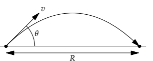
4.2.3 Projectile range

In the previous examples, only one variable was independent; changing it changed all the others. However, many problems contain multiple independent variables. An example is the range R of a rock launched at an angle \(\theta\) with speed v. The traditional derivation uses calculus. You solve for the position of the rock as a function of time, solve for the time when its height is zero (the ground level), and then insert that time into the horizontal position to find the range. This analysis is not wrong, but its result still seems like magic. I leave unsatisfied, thinking, “The result must be true. But I still do not know why.”

That “why” insight comes from proportional reasoning, which discards the nonessential complexity. Let’s begin with our doubling question.

How does doubling each of the independent variables affect the range?

The independent variables include the launch velocity v, the gravitational acceleration g (because gravity returns the rock to Earth), and the launch angle. However, angles do not fit so easily into proportional reasoning, so we won’t explore the role of \(\theta\) here (we will handle it in Section 8.2.2.1 using the tool of easy cases, or you can try Problem \(\PageIndex{8}\)).

Because the only forces are vertical, the rock’s horizontal velocity remains constant throughout its flight (an invariant!). Thus, the range is given by

\[R = \textrm{time aloft} \times \textrm{initial horizontal velocity}\]

The time aloft is determined by the initial vertical velocity, because gravity steadily reduces it (at the rate g):

\[\textrm{time aloft} \sim \frac{\textrm{initial vertical velocity}}{g}.\]

Exercise \(\PageIndex{7}\): Missing dimensionless prefactor

What is the missing dimensionless prefactor in the preceding expression for the time that the rock stays aloft?

Now double the launch velocity v. That change doubles the initial horizontal and vertical components of the velocity. Doubling the vertical component doubles the time aloft. Because the range is proportional to the horizontal velocity and to the time aloft, when the launch velocity doubles, the range quadruples. The scaling exponent connecting v to R is 2: \(R \: \propto \: v^{2}\).

What is the effect of doubling g?

Doubling g doesn’t change the horizontal velocity or the initial vertical velocity, but it halves the time aloft and therefore the range as well. The scaling exponent connecting g to R is −1: \(R \: \propto \: g^{-1}\)

The combined scaling relation, which gives the dependence of R on both g and v, is

\[R \: \propto \: \frac{v^{2}}{g}\]

Using v_x and v_y for the horizontal and vertical components of the launch velocity, the graphical representation of this reasoning is

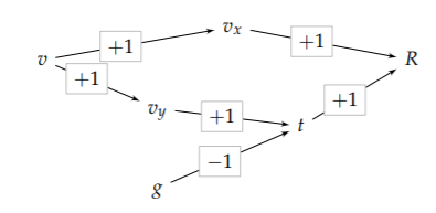
This graph shows a new feature: two independent variables, v and g. We’ll need to track the powers of v and g separately.

The range R has two incoming paths. The path via the horizontal velocity vx contributes +1 × +1 = +1 powers of v but no powers of g. The path via t also contributes +1 powers of v, and contributes −1 powers of g. The diagram compactly represents how R became proportional to \(v^{2}/g\).

The full range formula, including the launch angle \(\theta\) is

\[R \sim \frac{v^{2}}{g} \sin \theta \cos \theta\]

The dependence on v and g is just as we predicted.

The moral of this example is that you can derive and understand relations by ignoring constants of proportionality and instead concentrating on the scaling exponents. Furthermore, you can use this ability in order to spot mistakes: Just check each independent variable’s scaling exponent. For example, if someone proposes that projectile range R is proportional to \(v^{3}/g\), think, “The 1/g makes sense from the time aloft. But what about the v³? One power of v comes from the horizontal velocity and one power from the time aloft, which explains two powers of v. But where does the third power comes from? The range should instead contain v2/g.”

Exercise \(\PageIndex{8}\): Angular factors in projectile range

Explain the sin \(\theta\) and cos \(\theta\) factors by using the relation

\[\textrm{range} = \textrm{time aloft} \times \textrm{horizontal velocity}\]

4.2.4 Planetary surface gravity

Scaling, or proportional reasoning, connects independent to dependent variables. Often we have freedom in choosing the independent variables. Here is an example to show you how to use that freedom.

Assuming that planets are uniform spheres, how does g, the gravitational acceleration at the surface, depend on the planet’s radius R?

We seek the scaling exponent n in \(g \: \alpha \: R^{n}\). At the planet's surface, the gravitational force F on an object of mass m is \(GMm/R^{2}\), where G is Newton's constant, and M is the planet's mass. The gravitational acceleration g is F/m or GM/R² . Because G is the same for all objects, we pack light and eliminate G to make the proportionality

\[g \: \propto \: \frac{M}{R^{2}}\]

In this form, with mass M and radius R as the independent variables, the scaling exponent n is −2.

However, an alternative relation comes from noticing that the planet’s mass M depends on the planet’s radius R and density \(\rho\) as \(M \sim \rho R^{3}\) Then

\[g \: \propto \: \frac{\rho R^{3}}{R^{2}} = \rho R\].

In this form, with density and radius as the independent variables, the scaling exponent on R is now only 1.

Which scaling relation, with mass or density, is preferable?

Planets vary widely in their mass: from 3.3 × 10²³ kilograms (Mercury) to 1.9×10²⁷ kilograms (Jupiter), a range 4 decades wide (a factor of 10⁴). They vary greatly in their radius: from 7 ×10⁴ kilometers (Jupiter) down to 2.4× 10³ kilometers (Mercury), a range of a factor of 30. The quotient M/R² has huge variations in the numerator and denominator that mostly oppose each other. When there is change, look for what does not change—or, at least, what does not change as much. In contrast to masses, planetary densities vary from only 0.7 grams per cubic centimeter (Saturn) to 5.5 grams per cubic centimeter (Earth)—a range of only a factor of 8. The variations in planetary surface gravity are easier to understand using the planet’s radius and density rather than its radius and mass.

This result is general. Mass is an extensive quantity: When two objects combine, their masses add. Density, in contrast, is an intensive quantity. Adding more of a particular substance does not change its density. Using intensive quantities for the independent variables usually leads to more insightful results than using extensive quantities does.

Exercise \(\PageIndex{9}\): Distance to the Moon

The orbital period near the Earth’s surface (say, for a low-flying satellite) is roughly 1.5 hours. Use that information to estimate the distance to the Moon.

Exercise \(\PageIndex{10}\): Moon's angular diameter and radius

On a night with a full moon, estimate the Moon’s angular diameter—that is, the visual angle subtended by the Moon. Use that angle and the result of Problem \(\PageIndex{9}\) to estimate the Moon’s radius.

Exercise \(\PageIndex{11}\): Surface gravity on the Moon

Assuming that all planets (and moons) have the same density, use the radius of the Moon (Problem (\PageIndex{10}\)) to estimate its surface gravity. Then compare your estimate with the actual value and suggest an explanation for the discrepancy

Exercise \(\PageIndex{12}\): Gravitational strength inside a planet

Imagine a uniform, spherical planet with radius R. How does the gravitational acceleration g depend on r, the distance from the center of the planet? Give the scaling exponent when r <R and when r ≥ R, and sketch g(r).

Exercise \(\PageIndex{13}\): Making toast land butter-side up

As a piece of toast slides off a dining table (starting with almost no horizontal velocity), it picks up angular velocity. Once it leaves the table, its angular velocity remains constant. In everyday experience, a toast usually backflips (rotates 180^∘) by the time it hits the ground, and lands butter-side down. How high would tables have to be for a piece of toast to land butter-side up?