4.3: Scaling exponents in fluid mechanics

The preceding introductory examples may mislead you into thinking that proportional reasoning is useful only when we could also find the exact solution. As a counterexample, we return to that source of mathematical beauty but also misery, fluid mechanics, where exact solutions exist for hardly any situations of practical interest. To make progress, we need to discard complexity by focusing on the scaling exponents.

4.3.1: Falling cones

In Section 3.5.1, we used conservation reasoning to show that the drag force is given by

\[F_{drag} \sim \rho A_{cs} v^{2}.\]

In Section 3.5.2, we tested this result by correctly predicting the terminal speed of a falling paper cone. However, that experiment concerned only one cone of a particular size. A natural generalization of that experiment is to predict a cone’s terminal speed as a function of its size.

How does the terminal speed of a paper cone depend on its size?

Size is an ambiguous notion. It might refer to an area, a volume, or a length. Here, let's consider size to be the cone's cross-sectional radius r. The quantitative question is to find the scaling exponent n in \(v \: \propto \: r^{n}\), where v is the cone's terminal speed.

The doubling question is, "What happens to the terminal speed when we double r?" At the terminal speed, drag and weight mg balance:

\[\underbrace{\rho_{air} A_{cs} v^{2}}_{drag} \sim \underbrace{mg.}_{weight}\]

Therefore, the terminal speed is just what we found in Section 3.5.2:

\[v \sim \sqrt{\frac{mg}{\rho_{air}A_{cs}}}.\]

All cones feel the same g and \(\rho_{air}\), so we pack light and eliminate these variables to make the proportionality

\[v \: \propto \: \sqrt{\frac{m}{A_{cs}}}.\]

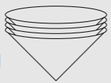
This result always surprises me. So I tried the experiment. I printed the cone template in Section 3.5.2 at 400-percent magnification (a factor of 4 increase in length), cut it out, taped the two straight edges together, and raced the small and big cones by dropping them from a height of about 2 meters. After a roughly 2-second fall, they landed almost simultaneously—within 0.1 seconds of each other. Thus, their terminal speeds are the same, give or take 5 percent.

Proportional reasoning triumphs again! Surprisingly, the proportional-reasoning result is much more accurate than the drag-force estimate \(\rho_{air}A_{cs}v^{2}\) on which it is based

How can predictions based on proportional reasoning be more accurate than the original relations?

To see how this happy situation arose, let’s redo the calculation but include the dimensionless prefactor in the drag force. With the dimensionless prefactor (shaded in gray), the drag force is

\[F_{drag} = \frac{1}{2}c_{d} \rho_{air}A_{cs}v^{2}, \]

where c_d is the drag coefficient (introduced in Section 3.2.1). The prefactor carries over to the terminal speed:

\[v = \sqrt{\frac{m}{\frac{1}{2}c_{d}A_{cs}}}.\]

Ignoring the prefactor decreases v by a factor of \(\sqrt{2/c_{d}}\). (For nonstreamlined objects, c_d ∼ 1, so the decrease is roughly by a factor of \(\sqrt{2}\).)

In contrast, in the ratio of terminal speeds \(v_{big}/v_{small}\), the prefactor drops out. Here is the ratio with the prefactors shaded in gray:

\[\frac{v_{big}}{v_{small}} = \sqrt{\frac{m_{big}}{\frac{1}{2} c_{d}^{big} A_{cs}^{big}}}/\sqrt{\frac{m_{small}}{\frac{1}{2}c_{d}^{small} A_{cs}^{small}}}.\]

As long as the drag coefficients c_d are the same for the big and small cones, they divide out from the ratio. Then the scaling result—that the terminal speed is independent of size—is exact, independent of the drag coefficient.

The moral, once again, is to build on what we know, rather than computing quantities that we do not need and that only clutter the analysis and thereby our thinking. Scaling relations bootstrap our knowledge. Here, if you know the terminal speed of the small cone, use that speed—and the scaling result that speed is independent of size—to find the terminal speed of the large cone. In the next section, we will apply this approach to estimate the fuel consumption of a plane.

Exercise \(\PageIndex{1}\): Taping the cones

The big cone, with twice the radius of the small cone, has four times the weight of paper. But what about the tape? If you tape along the entire radius of the cone template, how does the length of the tape compare between the large and small cones? How should you apply the tape in order to maintain the 4 : 1 weight ratio?

Exercise \(\PageIndex{2}\): Bigger and bigger cones

Further test the scaling relation \(v \: \propto \: r^{0}\) (terminal speed is independent of size) by building a huge cone from a template with four times the radius of the template for the small cone. Then race the small, big, and huge cones.

Exercise \(\PageIndex{3}\): Four cones versus one cone

Use the cone template in Section 3.5.2 (at 200-percent enlargement) to make five small cones. Then stack four of the cones to make one heavy small cone. How much faster will the four-cone stack fall in comparison to the single small cone? That is, predict the ratio of terminal speeds

\[\frac{v_{\textrm{four cones}}}{v_{\textrm{one cone}}}.\]

Then check your prediction by trying the experiment.

4.3.2 Fuel consumption of a Boeing 747 jumbo jet

In Section 3.5.4, we estimated the fuel consumption of automobiles. For the next example, we’ll estimate the fuel consumption of a Boeing 747 jumbo jet. Rather than repeating the structure of the automobile estimate in Section 3.5.4 but with parameters for a plane—which would be the brute-force approach—we will reuse the automobile estimate and supplement it with proportional reasoning.

A plane uses its fuel to generate energy to fight drag and to generate lift. However, for this estimate, forget about lift. At a plane’s cruising speed, lift and drag are comparable (as we will show in Section 4.6). Neglecting lift ignores only a factor of 2, because lift plus drag is twice the lift alone, and allows us to make a decent estimate without having to estimate the lift. Divide and conquer: Don’t bite off all the complexity at once!

The energy consumed fighting drag is proportional to the drag force:

\[E \: \alpha \: \rho_{air}A_{cs}v^{2}.\]

This scaling relation is shorthand for the following comparison between a plane and a car:

\[\frac{E_{plane}}{E_{car}} = \frac{\rho_{\textrm{air}}^{\textrm{cruising altitude}}}{\rho_{\textrm{air}}^{\textrm{sea level}}} \times \frac{A_{\textrm{cs}}^{\textrm{plane}}}{A_{\textrm{cs}}^{\textrm{car}}} \times (\frac{v_{\textrm{plane}}}{v_{\textrm{car}}})^{2}.\]

Thus, the energy-consumption ratio breaks into three ratio estimates.

What are reasonable estimates for the three ratios?

1. Air density. A plane’s cruising altitude is typically 35 000 feet or 10 kilometers, which is slightly above Mount Everest. At that height, mountain climbers require oxygen tanks, so the air, and oxygen, density must be significantly lower than it is at sea level. (Once you learn the reasoning tool of lumping, you can predict the density—see Problem 6.36.) The density ratio turns out to be roughly 3:

\[\frac{\rho_{\textrm{air}}^{\textrm{cruising altitude}}}{\rho_{\textrm{air}}^{\textrm{sea level}}} \approx \frac{1}{3}\]

The thinner air wins the plane a factor of 3 in fuel efficiency.

2. Cross-sectional area. To estimate the cross-sectional area of the plane, we need to estimate the width and height of the plane’s body; its wings are very streamlined, so they contribute negligible drag. When estimating lengths, let’s make our measuring rod (our unit) a person length. Using this measuring rod has two benefits. First, the measuring rod is easy for our gut to picture, because we feel our own size innately. Second, the lengths that we will measure will be only a small multiple of a person length. The numerical part of the quantity (for example, the 1.5 in “1.5 person lengths”) will be comparable to 1, and therefore also easy to picture. As a rule of thumb, ratios between 1/3 and 3 are easy to picture and feel in our gut because our mental number hardware is exact for the quantities 1, 2, and 3. We choose our measuring rods accordingly.

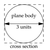
In applying the person-length measuring rod to the width of the plane’s body, I remember the comfortable days of regulated air travel. As a child, I would find three adjacent empty seats in the back of the plane and sleep for the whole trip (which explains why my parents insist that traveling with small children was easy). A jumbo jet is three or four such seat groups across—call it three person lengths—and its cross section is roughly circular. A circle is roughly a square, so the cross-sectional area is roughly 10 square person lengths:

\[(3 \textrm{ person lengths})^{2} \approx 10(\textrm{person length})^{2}.\]

Although we might worry that this estimate used too many approximations, we should do it anyway: It gives us a rough-and-ready value and allows us to make progress. Our goal is edible jam today, not delicious jam tomorrow!

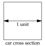
Now let's estimate the cross-sectional area of a car. In standard units, it's about 3 square meters, as we estimated in Section 3.5.4. But let's apply our person-sized measuring rod. From nocturnal activities in cars, you may have experienced that cars, uncomfortably, are about one person across. A car's cross section is roughly square, so the cross-sectional area is roughly 1 square person length.

Exercise \(\PageIndex{4}\): Comparing the cross-sectional areas

How well does 1 square person length match 3 square meters?

The ratio of cross-sectional areas is roughly 10; therefore, the plane’s larger cross-sectional area costs it a factor of 10 in fuel efficiency.

3. Speed.

A reason to fly rather than drive is that planes travel faster than cars. A plane travels almost at the speed of sound: 1000 kilometers per hour or 600 miles per hour. A car travels at around 100 kilometers per hour or 60 miles per hour. The speed ratio is roughly a factor of 10, so

\[(\frac{v_{plane}}{v_{car}})^{2} \approx 100.\]

The plane’s greater speed costs it a factor of 100 in fuel efficiency.

Now we can combine the three ratio estimates to estimate the ratio of energy consumptions:

\[\frac{E_{plane}}{E_{car}} \sim \underbrace{\frac{1}{3}}_{density} \times \underbrace{10}_{area} \times \underbrace{100}_{(speed)^{2}} \approx 300.\]

A plane should be 300 times less fuel efficient than a car—terrible news for anyone who travels by plane!

Should you therefore never fly again?

Our conscience is saved because a plane carries roughly 300 passengers, whereas a typical (Western) car is driven by one person to and from work. Therefore, per person, a plane and a car should have comparable fuel efficiencies: 30 passenger miles per gallon, as we estimated in Section 3.5.4, or 8 liters per 100 passenger kilometers.

Should you therefore never fly again? Our conscience is saved because a plane carries roughly 300 passengers, whereas a typical (Western) car is driven by one person to and from work. Therefore, per person, a plane and a car should have comparable fuel efficiencies: 30 passenger miles per gallon, as we estimated in Section 3.5.4, or 8 liters per 100 passenger kilometers.

\[\frac{216840 l}{13450 km} \times \frac{1}{416 passengers} \approx \frac{4l}{100 \: passenger \: km}.\]

Our proportional-reasoning estimate of 8 liters per 100 passenger kilometers is very reasonable, considering the simplicity of the method compared to a full fluid-dynamics analysis.

Exercise \(\PageIndex{5}\): Density of air by proportional reasoning

Make rough estimates of your own top swimming and cycling speeds, or use the data that a record 5-kilometer swim time is 56:16.6 (almost 1 hour). Thereby explain why the density of water must be roughly 1000 times the density of air. Why is this estimate more accurate when based on cycling rather than running speeds?

Exercise \(\PageIndex{6}\): Raindrop speed versus size

How does a raindrop’s terminal speed depend on its radius?

Exercise \(\PageIndex{7}\): Estimating an air ticket price from fuel cost

Estimate the fuel cost for a long-distance plane journey—for example, London to Boston, London to Cape Town, or Los Angeles to Sydney. How does the fuel cost compare to the ticket price? (Airlines do not pay many of the fuel taxes paid by ordinary motorists, so their fuel costs are lower than motorists’ fuel costs.)

Exercise \(\PageIndex{8}\): RElative fuel efficiency of a cycling

Estimate the fuel efficiency, relative to a car, of a bicyclist powered by peanut butter traveling at a decent speed (say, 10 meters per second or 20 miles per hour). Compare your estimate with your estimate in Problem 3.34.