4.5: Logarithmic Scales in Two Dimensions

Last updated
Save as PDF

Page ID: 24104

\( \newcommand{\vecs}[1]{\overset { \scriptstyle \rightharpoonup} {\mathbf{#1}} } \) \( \newcommand{\vecd}[1]{\overset{-\!-\!\rightharpoonup}{\vphantom{a}\smash {#1}}} \)\(\newcommand{\id}{\mathrm{id}}\) \( \newcommand{\Span}{\mathrm{span}}\) \( \newcommand{\kernel}{\mathrm{null}\,}\) \( \newcommand{\range}{\mathrm{range}\,}\) \( \newcommand{\RealPart}{\mathrm{Re}}\) \( \newcommand{\ImaginaryPart}{\mathrm{Im}}\) \( \newcommand{\Argument}{\mathrm{Arg}}\) \( \newcommand{\norm}[1]{\| #1 \|}\) \( \newcommand{\inner}[2]{\langle #1, #2 \rangle}\) \( \newcommand{\Span}{\mathrm{span}}\) \(\newcommand{\id}{\mathrm{id}}\) \( \newcommand{\Span}{\mathrm{span}}\) \( \newcommand{\kernel}{\mathrm{null}\,}\) \( \newcommand{\range}{\mathrm{range}\,}\) \( \newcommand{\RealPart}{\mathrm{Re}}\) \( \newcommand{\ImaginaryPart}{\mathrm{Im}}\) \( \newcommand{\Argument}{\mathrm{Arg}}\) \( \newcommand{\norm}[1]{\| #1 \|}\) \( \newcommand{\inner}[2]{\langle #1, #2 \rangle}\) \( \newcommand{\Span}{\mathrm{span}}\)\(\newcommand{\AA}{\unicode[.8,0]{x212B}}\)

Scaling relations, which are so helpful in understanding the physical and mathematical worlds, have a natural representation on logarithmic scales, the representation that we introduced in Section 3.1.3 whereby distances correspond to factors or ratios rather than to differences.

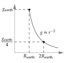
As an example, here is the gravitational strength g at a distance r from the center of a planet. Outside the planet, \(g \: \propto \: r^{-2}\), (the inverse-square law of gravitation). On linear axes, the graph of g versus r looks curved, like a hyperbola. However, its exact shape is hard to identify; the graph does not make the relation between g and r obvious. For example, let's try to represent our favorite scaling analysis: When r doubles, from, say R_Earthto 2R_Earth, the gravitational acceleration falls from g_Earth to g_Earth/4. The graph shows that g(2R) is smaller than g(R); unfortunately, the scaling is hard to extract from these points or from the curve.

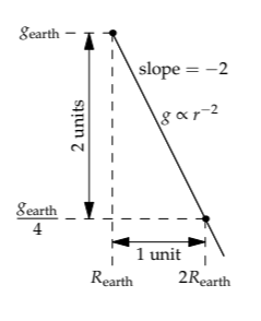
However, using logarithmic scales for both g and r—called log–log axes—makes the relation clear. Let’s try again to represent that when r doubles, the gravitational acceleration falls by a factor of 4. Call 1 unit on either logarithmic scale a factor of 2. The factor of 2 increase in r corresponds to moving 1 unit to the right. The factor of 4 decrease in g corresponds to moving 2 units downward. Therefore, the graph of g versus r is a straight line—and its slope is −2. On logarithmic scales, scaling relations turn into straight lines whose slope is the scaling exponent.

Exercise \(\PageIndex{1}\): Sketching gravitational field strength

Imagine, as in Problem 4.13, a uniform spherical planet with radius R. Sketch, on log–log axes, gravitational field strength g versus r, the distance from the center of the planet. Include the regions r<R and r ≥ R.

Many natural processes, often for unclear reasons, obey scaling relations. A classic example is Zipf’s law. In its simplest form, it states that the frequency of the kth most common word in a language is proportional to 1/k. The table gives the frequencies of the three most frequent English words. For English, Zipf’s law holds reasonably well up to k ~ 1000.

word	rank	frequency
the	1	7.0%
of	2	3.5
and	3	2.9

Zipf’s law is useful for estimation. For example, suppose that you have to estimate the government budget of Delaware, one of the smallest US states (Problem 4.30). A key step in the estimate is the population. Delaware might be the smallest state, at least in area, and it is probably nearly the smallest in population. To use Zipf’s law, we need the data for the most populous state. That information I happen to remember(information about the biggest item is usually easier to remember than information about the smallest item): The most populous state is California, with roughly 40 million people. Because the United States has 50 states, Zipf’s law predicts that the smallest state will have a population 1/50th of California’s, or roughly 1 million. This estimate is very close to Delaware’s actual population: 917 000.

Exercise \(\PageIndex{2}\): Government budget of Delaware

Based on the population of Delaware, estimate its annual government budget. Then look up the value and check your estimate.