4.6: Optimizing flight speed

With our skills in proportional reasoning, let’s return to the energy and power consumption in forward flight (Section 3.6.2). In that analysis, we took the flight speed as a given; based on the speed, we estimated the power required to generate lift. Now we can estimate the flight speed itself. We will do so by estimating the speed that minimizes energy consumption.

4.6.1 Finding the optimum speed

Flying requires generating lift and fighting drag. To find the optimum flight speed, we need to estimate the energy required by each process. The lift was the subject of Section 3.6.2, where we estimated the power required as

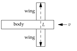
\[P_{lift} \sim \frac{(mg)^{2}}{\rho_{air}vL^{2}},\]

where m is the plane's mass, v is its forward velocity, and L is its wingspan. The lift energy required to fly a distance d is this power multiplied by the travel time d/v:

\[E_{lift} = P_{lift} \frac{d}{v} \sim \frac{(mg)^{2}}{\rho_{air}v^{2}L^{2}}d.\]

In fighting drag, the energy consumed is the drag force times the distance. The drag force is

\[F_{drag} = \frac{1}{2} c_{d} \rho_{air} v^{2} A_{cs},\]

where c_d is the drag coefficient. To simplify comparing the energies required for lift and drag, let's write the drag force as

\[F_{drag} = C \rho_{air}v^{2}L^{2},\]

where C is a modified drag coefficient: It doesn’t use the 1/2 that is part of the usual combination c_d/2, and it is measured relative to the squared wingspan L² rather than to the cross-sectional area A_cs.

For a 747, which drag coefficient, c_d or C, is smaller?

The drag force has two equivalent forms:

\[F_{drag} = \rho_{air} v^{2} \times \left\{ \begin{array}{ll} CL^{2}\\ \frac{1}{2}c_{d}A_{cs}. \end{array} \right.\]

Thus, \(CL^{2} = c_{d}A_{cs}/2\). For a plane, the squared wingspan L² is much larger than the cross-sectional area, so C is much smaller than c_d.

With the new form for F_drag, the drag energy is

\[E_{drag} = C \rho_{air} v^{2}L^{2}d,\]

and the total energy required for flying is

\[E_{total} \sim \underbrace{\frac{(mg)^{2}}{\rho_{air} v^{2} L^{2}}d}_{E_{lift}} + \underbrace{C \rho_{air} v^{2} L^{2}d.}_{E_{drag}}\]

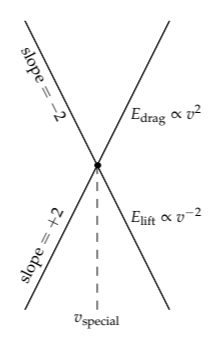
This formula looks intimidating because of the many parameters such as m, g, L, and \(\rho_{air}\). As our interest is the flight speed v (in order to find the total energy), let's use proportional reasoning to reduce the energies to their essentials: \(E_{drag} \: \alpha \: v^{2}\) and \(E_{lift} \: \alpha \: v^{-2}.\) On log-log axes, each relation is a straight line with slope +2 for drag and slope -2 for lift. Because the relations have different slopes, corresponding to different scaling exponents, their graphs must intersect.

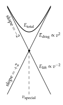
To interpret the intersection, let's incorporate a sketch of the total energy \(E_{total} = E_{drag} + E_{lift}\). At low speeds, the dominant consumer of energy is lift because of its v^-2 dependence, so the sketch of E_total follows E_lift. At high speeds, the dominant consumer of energy is drag because of its v² dependence, so the sketch of E_total follows E_drag. Between these extremes is an optimum speed that minimizes the energy consumption. (Because the axes are logarithmic, and \(\log(a + b) \neq \log a + \log b\), the sum of the two straight lines is not straight!) This optimum speed, marked v_special, is the speed at which E_drag and E_lift cross.

Why is the optimum right at the crossing speed, rather than faster or slower than the crossing speed?

Symmetry! Try Problem 4.31 and then look afresh at Section 3.2.3, where we minimized E_total without the benefit of log–log axes.

Flying faster or slower than the optimum speed means consuming more energy. That extra consumption cannot always be avoided. A plane is designed so that its cruising speed is its minimum-energy speed. At takeoff and landing, when it flies far below the minimum-energy speed, a plane must work harder to stay aloft, which is one reason that the engines are so loud at takeoff and landing (another reason is that the engine noise reflects off the ground and back to the plane).

The optimization constraint, that a plane flies at the minimum-energy speed, allows us to eliminate v from the total energy. As we saw on the graph, at the minimum-energy speed, the drag and lift energies are equal:

\[\underbrace{\frac{(mg)^{2}}{\rho_{air}v^{2}L^{2}}d}_{E_{lift}} \sim \underbrace{C \rho_{air} v^{2} L^{2} d,}_{E_{drag}}\]

or, solving for mg (and rejoicing that d canceled out),

\[mg \sim \sqrt{C} \rho_{air} v^{2}L^{2}\]

Now we could solve for v explicitly (and you get to find and use that solution in Problems 4.34 and 4.36). However, here we are interested in the total energy, not the flight speed itself. To find the energy without finding the speed, notice a reusable idea, an abstraction, within the right side of the equation for mg—which otherwise looks like a mess.

Namely, the mess contains \(\rho_{air}v^{2}L^{2}\), which is \(F_{drag}/C\). Therefore, when the plane is flying at the minimum-energy speed,

\[mg \sim \sqrt{C} \frac{F_{drag}}{C},\]

so

\[F_{drag} \sim \sqrt{C}mg.\]

Thanks to our abstraction and all the surrounding approximations, we learn a surprisingly simple relation between the drag force and the plane's weight, connected through the square root of our modified drag coefficient C.

The energy consumer by drag--which, within a factor of 2, is also the total energy--is the drag force times the distance d. Therefore, the total energy is given by

\[E_{total} \sim \underbrace{E_{drag}}_{F_{drag}d} \sim \sqrt{C} mgd.\]

By using an optimum flight speed, we have eliminated the flight speed v from the total energy.

Does the total energy depend in reasonable ways upon m, g, C, and d?

Yes! First, lift overcomes the weight mg; therefore, the energy should, and does, increase with mg. Second, a streamlined plane (low C) should use less energy than a bluff, blocky plane (high C); the energy should, and does, increase with the modified drag coefficient C. Finally, because the plane is flying at a constant speed, the energy should be, and is, proportional to the travel distance d.

4.6.2 Flight range

From the total energy, we can estimate the range of the 747—the distance that it can fly on a full tank of fuel. The energy is \(\sqrt{C} mgd\), so the range d is

\[d \sim \frac{E_{fuel}}{\sqrt{C} mg},\]

where \(E_{fuel} is the energy in the full tank of fuel. To estimate d, we need to estimate E_fuel, the modified drag coefficient C, and maybe also the plane's mass m.

How much energy is in a full tank of fuel?

The fuel energy is the fuel mass times its energy density (as an energy per mass). Let's describe the fuel mass relative to the plane's mass m, as a fraction \(\beta\) of the plane's mass: \(mass_{fuel} = \beta m\). Using \(\varepsilon_{fuel}\) for the energy density of fuel,

\[E_{fuel} = \beta m \varepsilon_{fuel}.\]

When we put this expression into the range d, the plane's mass m in E_fuel, which is the numerator of d, cancels the m in the denominator \(\sqrt{C} mg\). The range then simplifies to a relation independent of mass:

\[d \sim \frac{\beta \varepsilon_{fuel}}{\sqrt{C} g}.\]

For the fuel fraction \(\beta\), a reasonable guess for long-range flight is \(\beta\) ≈ 0.4: a large portion of the payload is fuel. For the energy density \(\varepsilon_{fuel}\), we learned in Section 2.1 that \(\varepsilon_{fuel}\) is roughly 4× 10⁷ joules per kilogram (9 kilocalories per gram). This energy density is what a perfect engine would extract. At the usual engine efficiency of one-fourth, \(\varepsilon_{fuel}\) becomes roughly 10⁷ joules per kilogram.

How do we find the modified drag coefficient C?

This estimate is the trickiest part of the range estimate, because C needs to be converted from more readily available data. According to Boeing, the manufacturer of the 747, a 747 has a drag coefficient of C' ≈ 0.022. As the prime symbol indicates, C' is yet another drag coefficient. It is measured using the wing area A_wing and uses the traditional 1/2:

This estimate is the trickiest part of the range estimate, because C needs to be converted from more readily available data. According to Boeing, the manufacturer of the 747, a 747 has a drag coefficient of C' ≈ 0.022. As the prime symbol indicates, C' is yet another drag coefficient. It is measured using the wing area A_wing and uses the traditional 1/2:

So we have three drag coefficients, depending on whether the coefficient is referenced to the cross-sectional area A_cs (the usual definition of c_d), to the wing area A_wing (Boeing’s definition of C')v or to the squared wingspan L² (our definition of C, which also lacks the factor of 1/2 that the others have).

To convert between these definitions, compare the three ways to express the drag force:

\[F_{drag} = \rho_{air} v^{2} \times \left\{ \begin{array}{ll} \frac{1}{2} C' A_{wing} \: (\textrm{Boeing's definition}), \\ CL^{2} \: (\textrm{our definition}), \\ \frac{1}{2} c_{d} A_{cs} \: (\textrm{the usual definition}). \end{array} \right. \]

From this comparison,

\[\frac{1}{2}C'A_{wing} = CL^{2} = \frac{1}{2}c_{d}A_{cs}.\]

The conversion from C' to C is therefore

\[C= \frac{1}{2} C' \frac{A_{wing}}{L^{2}}.\]

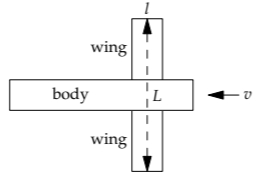
Using l for the wing’s front-to-back length, the wing area becomes \(A_{wing} = Ll\). Then the area ratio \(A_{wing}/L^{2}\) simplifies to l/L (the reciprocal of the wing aspect ratio), and the drag coefficient C simplifies to

\[C= \frac{1}{2} C' \frac{l}{L}.\]

For a 747, l ≈ 60 meters, and C' ≈ 0.222, so C ≈ 1/600:

\[C \sim \frac{1}{2} \times 0.022 \times \frac{10m}{60m} \approx \frac{1}{600}.\]

The resulting range is roughly 10 000 kilometers:

\[d \sim \frac{\overbrace{0.4}^{\beta} \times \overbrace{10^{7} \textrm{J kg} ^{-1}}^{\varepsilon_{fuel}}}{\underbrace{\sqrt{1/600}}_{\sqrt{C}} \times \underbrace{10 \textrm{ m s}^{-2}}_{g}} \approx 10^{7} m = 10^{4} km.\]

The actual maximum range of a 747-400 is 13,450 kilometers (a figure we used in Section 4.3.2): Our approximate analysis is amazingly accurate.

Exercise \(\PageIndex{1}\): Graphical interpretation of minimization using symmetry

In Section 3.2.3, we started with the general form for the total energy

\[E \sim \underbrace{\frac{A}{v^{2}}}_{E_{lift}} + \underbrace{B v^{2}}_{E_{drag}}\]

and found the optimum (minimum-energy) speed by constructing the following symmetry operation:

\[v \leftrightarrow \frac{\sqrt{A/B}}{v}.\]

On the log–log plot of the energies versus v, what is the geometric interpretation of this symmetry operation?

Exercise \(\PageIndex{2}\): Minimum-power speed

We estimated the flight speed v_E that minimizes energy consumption. We could also have estimated v_P, the speed that minimizes power consumption. What is the ratio v_P/v_E? Before doing an exact calculation, sketch P_lift, P_drag, and P_lift + P_drag (on log–log axes) and place v_P on the correct side of v_E. Then check your placement against the result of the exact calculation.

Exercise \(\PageIndex{3}\): Coefficient of lift

Just as we can define a dimensionless drag coefficient c_d, where

\[F_{drag} = \frac{1}{2} c_{d} \rho_{air} A v^{2},\]

we can define a dimensionless lift coefficient c_L, where

\[F_{lift} = \frac{1}{2} c_{L} \rho_{air} Av^{2},\]

where the area A here is usually the wing area. (The same formula structure shows up in drag and lift—abstraction!) Estimate c_L for a 747 in cruising flight.

4.6.3 Flight range versus size

In proportional reasoning, we ask, “How does one quantity change when we change an independent variable (for example, if we double an independent variable)?” Because flying objects come in such a wide range of sizes, a natural independent variable is size.

How does the flight range depend on the plane’s size?

Let's assume that all planes are geometrically similar--that is, that they have the same shape and differ only in their size. Now let's see how changing the plane's size changes the quantities in the range

\[d \sim \frac{\beta \varepsilon_{fuel}}{\sqrt{C}g}.\]

The gravitational acceleration g remains fixed. The fuel energy density \(\varepsilon_{fuel}\) and the fuel fraction \(\beta\) also remain fixed--which shows again the benefit of using intensive quantities, as we discussed in Section 4.2.4 when we made a scaling relation for planetary surface gravity. Finally, the drag coefficient C depends only on the plane's shape (on how streamlined it is), not on its size, so it too remains constant. Therefore, the flight range is independent of the plane's size!

A further surprise comes from comparing the range of planes with the range of migrating birds. The proportionality \(d \: \alpha \: \beta \varepsilon_{fuel}/\sqrt{C}\) is shorthand for the comparison

\[\frac{d_{plane}}{d_{bird}} = \frac{\beta_{plane}}{\beta_{bird}} \frac{\varepsilon_{plane}^{fuel}}{\varepsilon_{bird}^{fuel}} (\frac{C_{plane}}{C_{bird}})^{-1/2}.\]

The ratio of fuel fractions is roughly 1: For the plane, \(\beta\) ≈ 0.4; and a bird, having eaten all summer, is perhaps 40 percent fat (the bird’s fuel). The energy density in jet fuel and fat is similar, as is the efficiency of engines and animal metabolism (at about 25 percent). Therefore, the ratio of energy densities is also roughly 1. Finally, a bird has a similar shape to a plane, so the ratio of drag coefficients is also roughly 1. Therefore, planes and well-fattened migrating birds should have a similar maximum range, about 10 000 kilometers.

Let’s check. The longest known nonstop flight by an animal is 11 680 kilometers: made by a bar-tailed godwit tracked by satellite by Robert Gill and his colleagues [19] as the bird flew nonstop from Alaska to New Zealand!