6.3: Typical or characteristic values

Lumping not only simplifies numbers, where it is called rounding, it also simplifies complex quantities by creating an abstraction: the typical or characteristic value. We’ve used this form of lumping implicitly many times; now it’s time to discuss it explicitly, in order to appreciate its scope and to develop skill in applying it.

6.3.1 Estimating the population of the United States

Our first explicit example of a typical or characteristic value occurs in the following population estimate. Knowing a population is essential in many estimates about the social world, such as a country’s oil imports (Section 1.4), energy consumption, or per-capita land area (Problem 1.14). Here we’ll estimate the population of the United States by dividing it into two factors.

\[\textrm{US population} \sim N_{states} \times \textrm{ population of a typical US state.}\]

The first factor, N_states, everyone in America learns in school: N_states = 50. The second factor contains the lumping approximation. Rather than using all 50 different state populations, we replace each state with a typical state.

What is the population of a typical state?

A large state is California or New York, each of which has a megacity with a population in the several millions. A tiny state is Delaware or Rhode Island. In between is Massachusetts. Because I live there, I know that it has 6 million people. Taking Massachusetts as a typical state, the US population is roughly 50 × 6 million or 300 million. This estimate is more accurate than we deserve: The 2012 population is 314 million.

From this example, you can also see how lumping enhances symmetry reasoning: When there is change, look for what does not change (Section 3.1). Here, each state has its own population, so there’s plenty of change among the list of states. Lumping helps us find, or create, a quantity that does not change. We imagine a typical state, one that may not even exist (just as no family has the average of 2.3 children), and replace every state with this state. We’ve lumped away all the change—throwing away information in exchange for insight into the population of the country.

Problem 6.9: German federal states

The Federal Republic of Germany has 16 federal states. Pick one at random, multiply its population by 16, and compare that estimate with Germany’s population.

6.3.2 Lumping varying physical quantities: How high can animals jump?

Using typical or characteristic values allows us to reason out seemingly impossible questions while sitting in our armchairs. For practice, we’ll study how the jump height of an animal depends on its size. For example, should a person be able to jump higher than a locust?

The jump could be a running or a standing high jump. Both types are interesting, but the standing high jump teaches more about lumping. Therefore, imagine that the animal starts from rest and jumps directly upward.

Even with this assumption, the problem looks underspecified. The jump height depends at least on the animal’s shape, on how much muscle the animal has, and on the muscle efficiency. It is the kind of problem where lumping, a tool for making assumptions, is most helpful. We’ll use lumping and proportional reasoning to find the scaling exponent \(\beta\) in \(h \: \propto \: m \beta\), where h is the jump height and m is the animal’s mass (our measure of its size).

Finding a scaling exponent usually requires a physical model. You can often build them by imagining an extreme, unrealistic situation, and then asking yourself what physics prevents it from happening. Thus, why can’t we jump to the Moon? Because it demands a vast amount of energy, far beyond what our muscles can supply. The point to extract from this thought experiment is that jumping demands energy, which is supplied by muscles.

The appearance of supply and demand suggests, as in the estimate of the number of taxis in Boston (Section 3.4.1), that we equate the demand to the supply. Then we estimate each piece separately—divide and conquer.

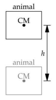
The energy demanded is the gravitational potential energy mgh. Here, g is the gravitational acceleration, and the jump height ℎ is measured as the vertical change in the animal’s center of mass (CM). Because all animals feel the same gravity, \(E_{demanded} = mgh\) simplifies to the proportionality \(E_{demanded} \: \propto \: mh\).

For the supplied energy, we again divide and conquer:

\[E_{supplied} \sim \textrm{muscle mass} \times \textrm{muscle energy density},\]

where the muscle energy density is the energy per mass that muscle can supply. This product already contains a lumping assumption: that all the muscles in an animal provide the same energy density. This assumption is reflected in the single approximation sign (~).

Even so, the result is not simple enough. Each species, and each individual within a species, will have its own muscle mass and energy density. Therefore, let’s make the further lumping assumption that all animals, even though they vary in muscle mass, share the same muscle energy density. The assumption is plausible because all muscles use similar biological technology (actin and myosin filaments). Fortunately, making this assumption is an approximation: Lumping throws away actual information, which is how it reduces complexity. With the assumption of a common energy density, the supplied energy becomes the simpler proportionality.

\[E_{supplied} \: \propto \: \textrm{muscle mass}.\]

The simplicity of this result reminds us that an approximate result can be more useful than an exact result.

The muscle mass also varies from animal to animal. Introducing a dimensionless prefactor and making another lumping approximation will manage that complexity. The dimensionless prefactor \(\alpha\) will be the fraction of an animal’s mass that is muscle:

\[m_{muscle} = \alpha m.\]

Alas, \(\alpha\) varies across species (compare a cheetah and a turtle), within a species, and within the lifetime of an individual—for example, my \(\alpha\) is dropping as I sit writing this book. If we account for all these variations, we will be overwhelmed by their complexity. Lumping rescues us: It gives us permission to assume that \(\alpha\) is the same for every animal. We replace the diversity of animals with a typical animal. This assumption is not as crazy as it might sound. It doesn’t mean that all animals have the same muscle mass. Rather, it means that all animals have the same fraction of muscle; as an example, for people, \(\alpha \sim 0.4\).

With this lumping assumption, \(m_{muscle} = \alpha m\) becomes the simpler proportionality \(m_{muscle} \: \propto \: m\). Because the supplied energy is proportional to the muscle mass, it is proportional to the animal’s mass:

\[E_{supplied} \: \propto \: m_{muscle} \: \propto \: m.\]

This result is as simple as we can hope for, and it depends on the right quantity, the animal’s mass. Now let’s use it to predict how an animal’s jump height depend on this mass.

Because the demanded energy and supplied energy are equal, and the demanded energy—the gravitational potential energy—is proportional to mh,

\[mh \: \propto \: m.\]

The common factor of m¹ cancels out, leaving h independent of m:

\[h \: \propto \: m^{0}.\]

All (jumping) animals should be able to jump to the same height!

The result always surprises me. My intuition, before doing the calculation, cannot decide how ℎ should behave. On the one hand, small animals seem strong: Ants can lift a mass many times their own body mass, whereas humans can lift only roughly their own body mass. However, my intuition also insists that people should be able to jump higher than locusts.

The data, from Scaling: Why Animal Size Is So Important [41, p. 178], contradict my intuition and confirm our lumping and scaling analysis. The mass spans more than eight orders of magnitude (eight decades, or a factor of 108), yet the jump height, as a change in the height of the center of mass, varies only by a factor of 3 (half a decade). On a log–log graph, the height-versus-mass line would have a slope less than 1/16. Our predicted scaling of constant jump height (\(h \: \alpha \: m^{0}\)), which corresponds to a slope of zero, is surprisingly accurate. The outliers, fleas and click beetles, are at the lighter end. (For an explanation, try Problem 6.10.) Furthermore, at the heavier end, locusts and humans, although differing by more than four orders of magnitude in mass, jump to almost exactly the same height.

	m	h
flea	0.5 mg	20cm
click beetle	40mg	30cm
locust	3g	59cm
human	70kg	60cm

A moral of this example is that lumping augments proportional reasoning. Proportional reasoning reduces complexity by showing us a notation for ignoring quantities that do not vary. For example, when all animals face the same gravitational field, then E_demanded=mgh simplifies to \(\E_{demanded} \: \alpha \: mh\). Alas, we live in the desert of the real, where “the same” is almost always only an approximation—for example, as with the energy density of muscle in different animals. Lumping rescues us. It gives us permission to replace these changing values with a single, constant, typical value—making the relations amenable to proportional reasoning.

Problem 6.10: Jumping fleas

The prediction of constant jump height seems to fail at small sizes: Larger animals jump about 60 centimeters, whereas fleas reach only 20 centimeters. In this problem, you evaluate whether air drag can explain the discrepancy.

a. As a lumping approximation, pretend that an animal is a cube with side length l, and assume that it jumps to a height h independent of its mass m. Then find the scaling exponent \(\beta\) in \(E_{drag}/E_{demanded} \: \alpha \: l \beta\), where E_drag is the energy consumed by drag and E_demanded is the energy needed in the absence of drag.

b. Estimate \(E_{drag}/E_{demanded}\) for a cubical human that can jump to 60 centimeters. Using the scaling relation, estimate it for a cubical flea. What is your judgment of drag as an explanation for the lower jump heights of fleas?

6.3.3 Period of an ideal spring

A surprising conclusion of dimensional analysis is that the period of a spring, or a small-amplitude pendulum, does not depend on its amplitude (Problem 5.14). However, the mathematical reasoning doesn’t give us the why; it doesn’t provide a physical insight. That insight comes from lumping, by using characteristic values. We’ll try it together by finding the period of a spring; you’ll practice by finding the period of a pendulum (Problem 6.11).

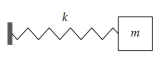
This kind of lumping, in exchange for providing physical insight, requires that we make a physical model. Here, a stretched or compressed spring exerts a force on and thereby accelerates the mass. If the spring is stretched to an amplitude \(x_{0}\), then the force is \(kx_{0}\) and the acceleration is \(kx_{0}/m\). This acceleration varies as the mass moves, so analyzing the motion usually requires differential equations. However, this acceleration is also a characteristic acceleration. It sets the scale forthe acceleration at all other times. If we replace the changing acceleration with this characteristic acceleration, the complexity vanishes. The problem becomes a constant-acceleration problem where \(a \sim kx_{0}/m\).

With a constant acceleration a for a time comparable to one period T, the mass moves a distance comparable to \(aT^{2}\), which is \(kx_{0}T^{2}/m\). When applying lumping and characteristic values, “comparable” is the verbal translation of the single approximation sign ~. As an equation, we would write

\[\textrm{distance} \sim aT^{2}.\]

Another useful translation is “of the order of”: The distance is of the order of \(aT^{2}\). Equivalently, the characteristic distance is \(aT^{2}\).

This characteristic distance must be comparable to the amplitude x₀. Thus,

\[x_{0} \sim \frac{kx_{0}T^{2}}{m}.\]

The amplitude \(x_{0}\) cancels out! Then the period is \(T \sim \sqrt{m/k}.\) Lumping thus provides the following explanation for why the period is independent of amplitude: As the amplitude and therefore the travel distance increase, the force and acceleration increase just enough to compensate, leaving the period unchanged.

Problem 6.11: Period of a small-amplitude pendulum using lumping

Use characteristic values to explain why the period of a (small-amplitude) pendulum is independent of the amplitude \(\theta_{0}\).

Problem 6.12: Period of a nonlinear spring

Imagine a nonlinear spring with force law \(F \: \alpha \: x^{n}\). Use lumping as follows to find how the period T varies with amplitude x₀.

a. Estimate a typical or characteristic acceleration.

b. At this acceleration, roughly how far does the mass travel in one period T?

c. This distance must be comparable to the amplitude x₀. Therefore, find the scaling exponent \(\alpha\) in \(T \: \alpha \: x^{\alpha}_{0}\) (where \(\alpha\) will be a function of the scaling exponent n in the force law). Then check your answer to Problem 5.17

6.3.4 Lumping derivatives

The preceding analysis of the period of a spring–mass system (Section 6.3.3) illustrates a general simplification: Using characteristic values, we can replace derivatives with algebra. The algebraic expression usually provides a physical model. As an example, let’s explain, physically, an acceleration that we derived by dimensional analysis in Section 5.1.1: the inward acceleration of an object moving in a circle.

Acceleration is the derivative of velocity: \(a = dv/dt\). Using the definition of derivative,

\[\frac{dv}{dt} \equiv \frac{\textrm{infinitesimal change in } v}{\textrm{(infinitesimal) time required to make this change in } v}.\]

Infinitesimal changes and times are difficult to picture, so an analysis based on calculus often does not help us see why a result is true.

A lumping approximation, by discarding complexity, can give this insight. A way to remember the lumping approximation, first use 6 = 6 to cancel the 6s in 16/64:

\[\frac{1 \cancel{6}}{\cancel{6} 4}= \frac{1}{4}.\]

The result is exact! Although this particular cancellation is dubious, it suggests the analogous lumping approximation \(d = d\). The resulting cancellation turns derivatives into algebra:

\[\frac{\cancel{d}v}{\cancel{d} t} \sim \frac{v}{t}.\]

What does \(v/t\) mean?

Lumping replaces “infinitesimal” with “characteristic”:

\[\frac{v}{t} \sim \frac{\textrm{characteristic change in } v}{\textrm{time required to make this change in } v}.\]

The numerator asks us to look at the changes in \(v\) and to represent them by a characteristic or typical change. The denominator is, as an abbreviation, often called the characteristic time, or time constant, and denoted \(\tau\).

In applying this approximation to circular motion, we have to distinguish the velocity vector v from its magnitude \(v\) (the speed). The speed, at least in constant-speed circular motion, never changes, so \(dv/dt\) itself is zero. We are interested in \(\vert d \textbf{v} \vert /dt\): the magnitude of the vector’s derivative, rather than the derivative of the vector’s magnitude. The lumped acceleration a is

\[a \sim \frac{\vert \textrm{characteristic change in } \textbf{v} \vert }{\textrm{time required to make this change in } \textbf{v}}.\]

The maximum change in v is reversing direction, from +v to -v. A characteristic change in v is v itself, or any value comparable to it. This range of possibilities is captured by the single approximation sign, which stands for “is comparable to.” With that notation,

\[\textrm{characteristic change in } \textbf{v} \sim textrm{v}.\]

Here is an example of such a change, showing the velocity vectors before and after the particle has rotated partway around the circle.

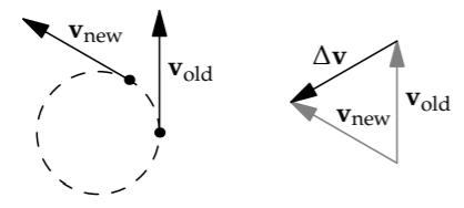
When v makes its significant change, from v_old to v_new, it produces a change in v comparable in magnitude to \(v\). The characteristic time \(\tau\)—the time required to make this change—is a decent fraction of a period of revolution. Because a full period is \(2 \pi r/v\), the characteristic time is comparable to \(r/v\). Using \(\tau\) to represent the characteristic time, and ~ to hide dimensionless prefactors, we write \(\tau \sim r/v\).

Here’s another way to arrive at \(\tau \sim r/v\). If the triangle of v_old, v_new, and \(\Delta \textbf{v}\) is an equilateral triangle, then it corresponds to the particle rotating 60^∘ around the circle, which is almost exactly 1 radian. Because 1 radian creates an arc of length r (the same proportionality tells us that \(2 \pi\) radians produces the circumference \(2 \pi r\)), the travel time is \(r/v\), and \(\tau \sim r/v\). Then the acceleration is roughly \(v^{2}/r\):

\[a \sim \frac{v}{\tau} \sim \frac{v}{r/v} = \frac{v^{2}}{r}.\]

This equation encapsulates a physical, proportional-reasoning explanation of \(a= v^{2}/r\). Namely, in circular motion, the velocity vector changes direction significantly in approximately 1 radian of rotation. This motion requires a time \(\tau \sim r/v\). Therefore, the circular acceleration a contains two factors of \(v\)—one factor from the \(v\) itself and one factor from the time in the denominator—and it contains 1/r, also from the time in the denominator.

6.3.5 Simplifying with characteristic values: Yield of the first atomic blast

In Section 5.2.2, we used dimensional analysis to estimate the yield of an atomic blast. We accurately predicted that the blast energy E is related to the blast radius ​​​​​​R the air density \(\rho\):

\[E \sim \frac{\rho R^{5}}{t^{2}},\]

where t is the time since the blast. However, dimensional analysis, as a mathematical argument, does not give a physical explanation for its results, which can often feel like magic. Lumping explains the magic by helping us analyze a physical model—a model whose analysis would otherwise be absurd in its complexity.

The physical model is that the blast increases the thermal energy of the air molecules, thus increasing the speed of sound—which is the speed at which the blast expands. Using this model exactly requires setting up and solving differential equations, as Taylor did [44]. Lumping, by turning calculus into algebra, simplifies the equations without discarding their physical meaning.

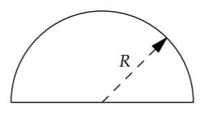
The first step is to estimate the thermal energy. It comes almost entirely from the hot fireball—that is, from the blast energy. This energy is spread unevenly over the blast, with a higher energy density nearer the blast center and a lower density farther away. For the lumping approximation, smear the blast energy E evenly throughout a sphere of radius R. This sphere’s volume is comparable to \(R^{3}\), so the typical or characteristic energy density is \(\varepsilon \sim E/R^{3}\)

The next step is to use this energy density to estimate the speed of sound c_s. As we discussed in Section 5.4.1, the speed of sound is comparable to the thermal speed, so

\[c_{s} \sim \sqrt{\frac{k_{B}T}{m}},\]

where \(k_{B}T\) is the approximate thermal energy of one air molecule and m is the mass of one air molecule.

To connect this speed to the energy density \(\varepsilon\), let’s convert energy per molecule into energy per volume, by multiplying \(k_{B}T\) by the number density n (the number of air molecules per volume). The result is \(nk_{B}T\), which is the thermal and therefore roughly the blast energy density \(\epsilon \sim E/R^{3}\).

To be fair, we also multiply the denominator m by n. This step converts mass per molecule into mass per volume, which gives the density \(\rho\):

\[\underbrace{\frac{\textrm{mass}}{\textrm_{molecule}}}_{m} \times \underbrace{\frac{\textrm{molecules}}{\textrm{volume}}}_{n} = \underbrace{\frac{\textrm{mass}}{\textrm{volume}}}_{\rho}.\]

Therefore, the speed of sound is comparable to \(\sqrt{E/\rho R^{3}}\):

\[c_{s} \sim \sqrt{\frac{nk_{B}T}{nm}} \sim \sqrt{\frac{E/R^{3}{\rho}} = \sqrt{\frac{E}{\rhoR^{3}}}.\]

This speed is the rate at which the blast expands.

Based on this speed, how large should the blast be after time \(t\)?

Because the energy density and therefore the sound speed decreases as R increases, the blast radius is not simply the speed at the time t multiplied by the time. But we can make a further lumping approximation: that the typical or characteristic speed, for the entire time t, is \(\sqrt{E/\rho R^{3}}.\) In evaluating this speed, we'll use the radius R at time t as the characteristic radius.

\[\underbrace{\textrm{blast radius}}_{R} \sim \underbrace{\textrm{characteristic speed}}_{c_{s} \sim \sqrt{E/\rho R^{3}}} \times \underbrace{\textrm{time}}_{t}.\]

The solution for the blast energy E is \(E \sim \rho R^{5}/t^{2}\), as we found using dimensional analysis. Lumping complements that mathematical reasoning with a physical model.