6.5: Quantum Mechanics

When we introduced quantum mechanics to estimate the size of hydrogen (Section 5.5.1), it was an actor in dimensional analysis. There, quantum mechanics merely contributed a new constant of nature \(\hbar\). This contribution was mathematical. By using lumping to introduce quantum mechanics, we will gain a physical intuition for the effect of quantum mechanics.

6.5.1 Particle in a box: Size of neutron stars

In mechanics, the simplest useful model is motion in a straight line at constant acceleration (which includes constant velocity). This model underlies numerous analyses—for example, the lumping analysis of a pendulum period (Section 6.3.3). In quantum mechanics, the simplest useful model is a particle confined to a box. Let’s give the particle a mass m and the box a width a.

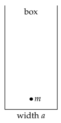
What is the lowest possible energy of the particle—that is, its ground-state energy?

Because this box can be a lumping model for more complex problems, this energy will help us explain the binding energy of hydrogen. A lumping analysis starts with Heisenberg’s uncertainty principle:

\[\Delta p \Delta x \sim \hbar.\]

Here, \(\Delta p\) is the spread (the uncertainty) in the particle’s momentum, \(\Delta x\) is the spread in its position, and \(\hbar\) is the quantum constant. If we know the position precisely (that is, if the uncertainty \(\Delta x\) is tiny), then the momentum uncertainty \(\Delta p\) must be large in order to make the product \(\Delta p \Delta x\) comparable to \(\hbar\). In contrast, if we hardly know the position (\(\Delta x\) is large), then the momentum uncertainty \(\Delta p\) can be small. This relation is the physical contribution of quantum mechanics.

Let’s apply it to the particle in the box. The particle could be anywhere in the box, so its position uncertainty \(\Delta x\) is comparable to the box width a:

\[\Delta x \sim a.\]

Because of the uncertainty principle, the consequence of confining the particle to the box implies a momentum uncertainty \(\hbar /a\):

\[\Delta p \sim \frac{\hbar}{\Delta x} \sim \frac{\hbar}{a}.\]

This momentum corresponds to a kinetic energy \(E \sim (\Delta p)^{2}/m\). As a consequence, the particle acquires an energy, called the confinement energy:

\[E \sim \frac{\hbar ^{2}}{ma^{2}}.\]

This simple result enables us to estimate the radius of a neutron star: a star without any nuclear fusion (which normally resists gravity) and heavy enough that gravity has collapsed the protons and electrons into neutrons. The atomic structure is gone, and the star is one giant, neutral nucleus (except in the crust, where gravity is not strong enough to make neutrons).

Problem 6.31: Dimensional analysis for the size of a neutron star

Use dimensional analysis to find the radius R of a neutron star of mass M.

Two physical effects compete: Gravity tries to crush the star; and quantum mechanics, armed with the uncertainty principle, resists by penalizing confinement. To begin quantifying these effects, let the star have radius R and contain N neutrons, so it has mass \(M= Nm_{n}\).

Gravity’s contribution to crushing the star is reflected in the star’s gravitational potential energy

\[E_{potential} \sim \frac{GM^{2}}{R}.\]

This energy is negative: Gravity is happier (the energy is lower) when R is smaller. Here, the minus sign is incorporated into the single approximation sign ~.

For the other side of the competition, we confine each neutron to a box. To find the box width a, imagine the star as a three-dimensional cubic lattice of neutrons. Because the star contains N neutrons, the lattice is \(N^{1/3} \times N^{1/3} \times N^{1/3}\). Each side has length comparable to R, so \(a N^{1/3} \sim R\) and \(a \sim R/N^{1/3}\).

Each neutron gets a confinement (kinetic) energy \(\hbar ^{2}/m_{n}a^{2}\). For all the N neutrons together, and using \(a \sim R/N^{1/3}\),

\[E_{kinetic} \sim N\frac{\hbar^{2}}{m_{n}a^{2}} \sim N^{5/3} \frac{\hbar ^{2}}{m_{n}R^{2}}.\]

In terms of the known masses M and m_n (instead of N), the total confinement energy is

\[E_{kinetic} \sim \frac{M^{5/3}}{m_{n}^{8/3}} \frac{\hbar ^{2}}{R^{2}}.\]

The kinetic energy is proportional to \(R^{-2}\), whereas the potential energy is proportional to \(R^{-1}\). On log–log axes of energy versus radius, the kinetic energy is a straight line with a −2 slope, and the potential energy is a straight line with a −1 slope. Because the slopes differ, the lines cross. The radius where they cross, which is roughly the radius that minimizes the total energy, is also roughly the radius of the neutron star. (We used the same reasoning in Section 4.6.1, to find the speed that minimized the energy required to fly.)

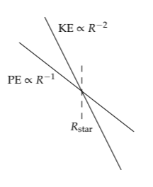
With all the constants included, the crossing happens when R satisfies

\[\frac{GM^{2}}{R} \sim \frac{M^{5/3}}{m_{n}^{8/3}} \frac{\hbar ^{2}}{R^{2}}.\]

The radius of the neutron star is then

\[R \sim \frac{\hbar ^{2}}{GM^{1/3}m_{n}^{8/3}}.\]

If the Sun, with a mass of 2×10³⁰ kilograms, became a neutron star, it would have a radius of roughly 3 kilometers:

\[R \sim \frac{(10^{-34} kg m^{2} s^{-1})^{2}}{7 \times 10^{-11} kg^{-1} m^{3} s^{-2} \times (2 \times 10^{30} kg)^{1/3} \times (1.6 \times 10^{-27} kg)^{8/3}} \sim 3 km.\]

The true neutron-star radius for the Sun, after including the complicated physics of a varying density and pressure, is approximately 10 kilometers. (In reality, the Sun’s gravity wouldn’t be strong enough to crush the electrons and protons into neutrons, and it would end up as a white dwarf rather than a neutron star. However, Sirius, the subject of Problem 6.32, is massive enough.)

Here is a friendly numerical form that incorporates the 10-kilometer information. It makes explicit the scaling relation between the radius and the mass, and it measures mass in the convenient units of the solar mass.

\[R \approx 10 km \times (\frac{M_{Sun}}{M})^{1/3}.\]

Our analysis, which used several lumping approximations and neglected many dimensionless constants throughout, predicted a prefactor of 3 kilometers instead of 10 kilometers. An error of a factor of 3 is a worthwhile tradeoff. We avoid the complicated analysis of a quantum fluid of electrons, protons, and neutrons, and still gain insight into the essential physical idea: The size of a neutron star results from a competition between gravity and quantum mechanics. (You will find many insightful astrophysical scalings in an article on the “Astronomical reach of fundamental physics” [5].)

Problem 6.32: Sirius as a neutron star

Sirius, the brightest star in the night sky, has a mass of 4 × 10³⁰ kilograms. What would be its radius as a neutron star?

6.5.2 Hydrogen by lumping

Having practiced quantum mechanics and lumping in the large (a neutron star), let’s go to the small: We’ll use lumping to complement the dimensional-analysis estimate of the size of hydrogen in Section 5.5.1. Its size is the radius of the orbit with the lowest energy. Because the energy is a sum of the potential energy from the electrostatic attraction and the kinetic energy from quantum mechanics, hydrogen is analogous to a neutron star, where quantum mechanics competes instead against gravitation. Partly because electrostatics is much stronger than gravity (Problem 6.34), hydrogen is very tiny.

For now, let the hydrogen atom have an unknown radius r. As a lumping approximation, the complicated electrostatic potential becomes a box of width r. Then the electron’s momentum uncertainty is \(\Delta p \sim \hbar /r\) and its confinement energy is \(\hbar ^{2}/m_{3}r^{2}\):

\[E_{kinetic} \sim \frac{(\Delta p)^{2}}{m_{e}} \sim \frac{\hbar ^{2}}{m_{e}r^{2}}.\]

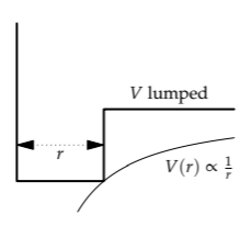
This energy competes against the electrostatic energy, whose estimate also requires a lumping approximation. For in quantum mechanics, an electron is not at any definite location. Depending on your interpretation of quantum mechanics, and speaking roughly, it is either smeared over the box, or it has a probability of being anywhere in the box. On either interpretation, calculating the potential energy requires an integral. However, we can approximate it by using lumping: The electron’s typical, or characteristic, distance from the proton is simply r, the radius of hydrogen (which is the size of the lumping box).

Then the potential energy is the electrostatic energy of a proton and electron separated by r:

\[E_{potential} \sim -\frac{e^{2}}{4 \pi \epsilon_{0}r}.\]

The total energy is their sum

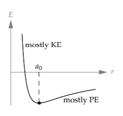
\[E = E_{potential} + E_{kinetic} \sim - \frac{e^{2}}{4 \pi \varepsilon_{0} r} + \frac{\hbar ^{2}}{m_{e}r^{2}}.\]

The electron adjusts r to minimize this energy. As we learned in the analysis of lift (Section 4.6.1), when two terms with different scaling exponents compete, the minimum occurs where the terms are comparable. (In Section 8.3.2.2, we’ll return to this example with the additional tool of easy cases and also sketch the energies on log–log axes.) Using the Bohr radius a₀ as the separation of minimum energy, comparability means

\[\underbrace{\frac{e^{2}}{4 \pi \varepsilon_{0}a_{0}}}_{E_{potential}} \sim \underbrace{\frac{\hbar ^{2}}{m_{e}a^{2}_{0}}}_{E_{kinetic}}.\]

The Bohr radius is therefore

\[a_{0} \sim \frac{\hbar^{2}}{m_{e}(e^{2}/4 \pi \varepsilon_{0})},\]

as we found in Section 5.5.1 using dimensional analysis. Now we also get a physical model: The size of hydrogen results from competition between electrostatics and quantum mechanics

Problem 6.33: Minimizing the energy in hydrogen using symmetry

Use symmetry to find the minimum-energy separation in hydrogen, where the total energy has the form

\(\frac{A}{r^{2}} - \frac{B}{r}.\)

(See Section 3.2.3 for related examples.)

Problem 6.34: Electrostatics versus gravitation

Estimate the ratio of the gravitational to the electrostatic force in hydrogen. What are the similarities and differences between this estimate and the estimate that you made in Problem 2.15?