7.2: Plausible ranges - Why divide and conquer works

The Bayesian understanding of probability as degree of belief will show us why divide-and-conquer reasoning (Chapter 1) works. We’ll see how it increases our confidence in an estimate and decreases our uncertainty as we analyze a divide-and-conquer estimate in slow motion.

7.2.1 Land area of the United Kingdom

The estimate will be the land area of the United Kingdom, which is where I was born and later spent many years. So I have some implicit knowledge of the area, but I don’t know it explicitly. The estimate therefore serves as a model for the common situation where we know more than we think we do and need to bring out and use that knowledge.

To make the initial estimate, the baseline against which to compare the divide-and-conquer estimate, I talk to my gut using the rubric of Section 1.6. For the lower end of my range, 10⁴ square kilometers feels right: I would be fairly surprised if the area were smaller. For the upper end, 10⁷ square kilometers feels right: I would be fairly surprised if the area were larger. Combining the endpoints, I would be mildly surprised if the area were smaller than 10⁴ square kilometers or greater than 10⁷ square kilometers. The wide range, spanning three orders of magnitude, reflects the difficulty of estimating an area without using divide-and-conquer reasoning.

My confidence in the gut estimate is my probability for the hypothesis H:

\[H \equiv \textrm{The UK's land area lies in the range } 10^{4} ... 10^{7} km^{2}.\]

This probability assumes, or is based on, my background knowledge K:

\[K \equiv \textrm{what I know about the area } before { using divide and conquer.}\]

My confidence or degree of belief in the guess is the conditional probability Pr (H ∣ K): the probability that the area lies in the range, based on my knowledge before applying divide-and-conquer reasoning. Alas, no algorithm is known for computing a probability based on such complicated background information. The best that we can do is to introspect: to hold a further gut discussion. This discussion concerns not the area itself, but rather the degree of belief about the range 10⁴…10⁷ square kilometers.

My gut chose the range for which I would feel mild surprise, but not shock, to learn that the area lies outside it. The surprise implies that the probability Pr (H ∣ K) is larger than 1/2: If Pr (H ∣ K) were less than 1/2, I would be surprised to find the area inside the range. The mildness of the surprise suggests that Pr(H ∣ K) is not much larger than 1/2. The probability feels like 2/3. The corresponding odds are 2:1; I'd give 2-to-1 odds that the area lies within the plausible range. With a further assumption of symmetry, so that the area's falling below and above the range are equally likely, the plausible range represents the following probabilities:

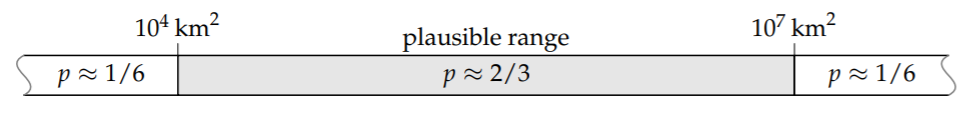
where the wavy lines at the ends indicate that the left and right ranges extend down to zero and up to infinity, respectively.

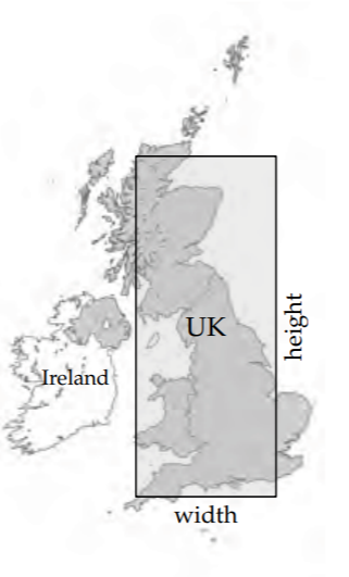
Now let’s see how a divide-and-conquer estimate changes the plausible range. To make this estimate, lump the area into a rectangle with the same area and aspect ratio as the United Kingdom. My own best-guess rectangle is superimposed on the map outline of the United Kingdom. Its area is the product of its width and height. Then the area estimate divides into two simpler estimates.

1. Lumped width. Before I ask my gut for the plausible range for the width, I prepare by reviewing my knowledge of the width. Crossing the United Kingdom the south, say from London to Cornwall, takes maybe 4 hours by car. But much of the United Kingdom is thinner, so the average, or lumped, width corresponds to maybe hours of driving. My gut is content with the range miles or kilometers:

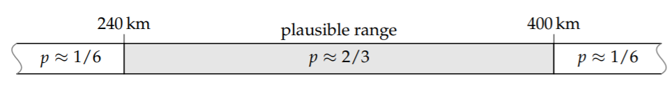
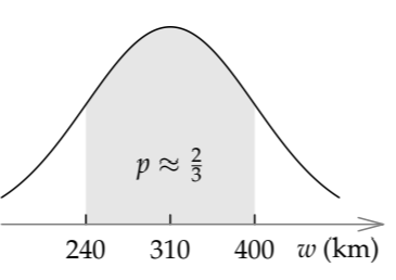
On a logarithmic scale, which is the correct scale for positive quantities such as the width and height, the midpoint of the range is \(\sqrt{240 \times 400}\) or 310 kilometers. It is my best estimate of the width.

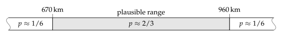
2. Lumped height. The train journey from London in the south of England to Edinburgh 5 in Scotland, in 80 the northern part of the United Kingdom, takes about hours at, say, miles per hour. In addition to these miles, there’s more latitude in Scotland north of Edinburgh and some 400 in England south of London. Thus, my gut estimate for the height of the lumping rectangle is 500 miles. This distance is the midpoint of my plausible range for the height.

The estimate feels accurate to plus or minus 20 percent (roughly ±100 miles). On a logarithmic (or multiplicative) scale, the range would be roughly a factor of 1.2 on either side of midpoint:

\[\underbrace{420}_{500/1.2} ... \underbrace{600}_{500 \times 1.2} miles.\]

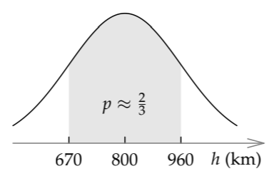
(A more accurate value for 500/1.2 is 417, but there’s little reason to strive for such accuracy when these endpoints are rough estimates anyway.) In metric units, the range is 670…960 kilometers, with a midpoint of 800 kilometers. Here is its probability interpretation:

The next step is to combine the plausible ranges for the height and the width in order to make the plausible range for the area. A first approach, because the area is the product of the width and height, is simply to multiply the endpoints of the width and height ranges:

\[A_{min} \approx 240 km \times 670 km \approx 160000 km^{2}; \\ A_{max} \approx 400 km \times 960 km \approx 380000 km^{2}.\]

The geometric mean (the midpoint) of these endpoints is 250000 square kilometers.

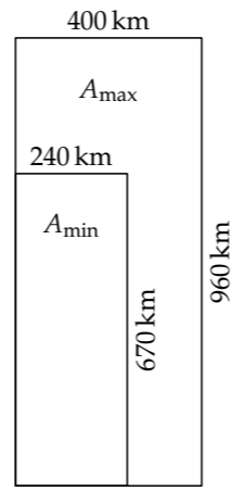
Although reasonable, this approach overestimates the width of the plausible range—a mistake that we’ll correct shortly. However, even this overestimated range spans only a factor of 2.4, whereas my starting range of 10⁴…10⁷ square kilometers spans a factor of 1000. Divide-and-conquer reasoning has significantly narrowed my plausible range by replacing a quantity about which I have vague knowledge, namely the area, with quantities about which I have more precise knowledge.

The second bonus is that subdividing into many quantities carries only a small penalty, smaller than suggested by simply multiplying the endpoints. Multiplying the endpoints produces a range whose width is the product of the two widths. But this width assumes the worst. To see how, imagine an extreme case: estimating a quantity that is the product of ten independent factors, each of which you know to within a factor of 2 (in other words, each plausible range spans a factor of 4). Does the plausible range for the final quantity span a factor of 4¹⁰ (approximately 10⁶)? That conclusion is terribly pessimistic. More likely, several of the ten estimates will be too large and several will be too small, allowing many errors to cancel.

Correctly computing the plausible range for the area requires a complete probabilistic description of the plausible ranges for the width and height. With it we could compute the probability of each possible product. That description is, somewhere, available to the person giving the range. But no one knows how to deduce such a complete set of probabilities based on the complex, diffuse, and seemingly contradictory information lodged in a human mind.

A simple solution is to specify a reasonable probability distribution. We’ll use the log-normal distribution. This choice means that, on a logarithmic scale, the probability distribution is a normal distribution, also known as a Gaussian distribution.

Here’s the log-normal distribution for my gut estimate of the height of the UK lumping rectangle. The horizontal axis is logarithmic: Distances correspond to ratios rather than differences. Therefore, 800 rather than 815 kilometers lies halfway between 670 and 960 kilometers. These endpoints are a factor of 1.2 smaller or larger than the midpoint. The peak at 800 kilometers reflects my belief that 800 kilometers is the best guess. The shaded area of 2/3 quantifies my confidence that the true height lies in the range 670…960 kilometers.

We use the log-normal distribution for several reasons. First, our mental hardware compares quantities using ratio rather than absolute difference. (By “quantity,” I mean inherently positive values, such as distance, rather than signed values such as position.) In short, our hardware places quantities on a logarithmic scale. To represent our thinking, we therefore place the distribution on a logarithmic scale.

Second, the normal distribution, which has only two parameters (midpoint and width), is simple to describe. This simplicity helps us when we translate our internal gut knowledge into the distribution’s parameters. From our gut estimates of the lower and upper endpoints, we just find the corresponding midpoint and width (on a logarithmic scale!): The midpoint is the geometric mean of the two endpoints, and the width is the square root of the ratio between the upper and lower endpoints.

Third, normal distributions combine simply. When we add two quantities represented by a normal distribution, their sum is also represented by a normal distribution.

On the other hand, the normal distribution does not represent all aspects of our gut knowledge. In particular, the tails of the normal distribution are too thin, reflecting an unrealistically high confidence that our estimate does not contain a huge error. Fortunately, for our analyses, this problem is not so significant, because we will concern ourselves with the location and width of the central region, and not take the thin tails too seriously. With that caveat, we’ll represent our plausible range as a normal distribution on a logarithmic scale: a log-normal distribution.

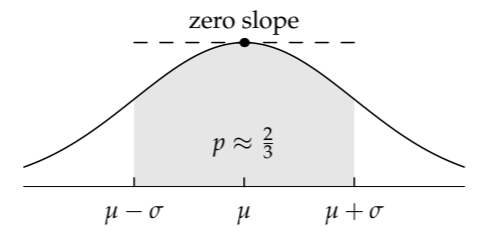
Here is the other log-normal distribution, for the width of the UK lumping rectangle. The shaded range is the so-called one-sigma range \(\mu - \sigma\) to \(\mu + \sigma\), where \(\mu\) is the midpoint (here, 310 kilometers) and \(\sigma\) is the width, measured as a distance on a logarithmic scale. In a normal distribution, the one-sigma range contains 68 percent of the probability—conveniently close to 2/3. When we ask our plausible ranges to contain a 2/3 probability, we are estimating a one-sigma range.

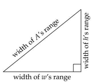
The two log-normal distributions supply the probabilistic description required to combine the plausible ranges. The rules of probability theory (Problem 7.5) produce the following two-part recipe.

1. The midpoint of the plausible range for the area A is the product of the midpoint of the plausible ranges for h and w. Here, the height midpoint is 800 kilometers and the width midpoint is 310 kilometers, so the area midpoint is roughly 250 000 square kilometers:

\[\underbrace{800km}_{h} \times \underbrace{310km}_{w} \approx 250000 km^{2}.\]

2. To compute the plausible range’s width or half width, first express the individual half widths (the \(\sigma\) values) in logarithmic units. Convenient units include factors of 10, also known as bels, or the even-more-convenient decibels. A decibel, whose abbreviation is dB, is one-tenth of a factor of 10. Here is the conversion between a factor \(f\) and decibels:

\[\textrm{number of decibels} = 10 log_{10} f.\]

For example, a factor of 3 is close to 5 decibels (because 3 is almost one-half of a power of ten), and a factor of 2 is almost exactly 3 decibels.

(These decibels are slightly more general than the acoustic decibels introduced in Problem 3.10: Acoustic decibels measure energy flux relative to a reference value, usually 10⁻¹² watts per square meter. Both kinds of decibels measure factors of 10, but the decibels here have no implicit reference value.)

In decibels, bels, or any logarithmic unit, the half width (the \(\sigma\)) of the product’s range is the Pythagorean sum of the individual half widths (the \(\sigma\) values). Using \(\sigma_{x}\) to represent the half width of the plausible range for the quantity x, the recipe is

\[\sigma_{A} = \sqrt{\sigma_{h}^{2} + \sigma_{w}^{2}}.\]

Let’s apply this recipe to our example. The plausible range for the height (ℎ) was 800 kilometers give or take a factor of 1.2. On a logarithmic scale, distances are measured by ratios or factors, so think of a range as “give or take a factor of” rather than as “plus or minus” (a description that would be appropriate on a linear scale). A factor of 1.2 is about ±0.8 decibels:

\[10 log_{10} 1.2 \approx 0.8.\]

Therefore, \(\sigma_{h} \approx 0.8\) decibels.

The plausible range for the width (w) was roughly 310 kilometers give or take a factor of 1.3. A factor of 1.3 is ±1.1 decibels:

\[10 log_{10} 1.3 \approx 1.1.\]

Therefore, \(\sigma_{w} \approx 1.1\) decibels.

The Pythagorean sum of \(\sigma_{h}\) and \(\sigma_{w}\) is approximately 1.4 decibels:

\[\sqrt{0.8^{2} + 1.1^{2}} \approx 1.4.\]

As a factor, 1.4 decibels is, coincidentally, approximately a factor of 1.4:

\[10^{1.4/10} \approx 1.4.\]

Because the midpoint of the plausible range is 250000 kilometers, the UK land area should be 250000 square kilometers give or take a factor of 1.4. Retaining a bit more accuracy, it is a factor of 1.37.

\[\underbrace{180000}_{/1.37} ... \underbrace{250000}_{\textrm{midpoint}} ... \underbrace{340000}_{\times 1.37} km^{2}.\]

As a probability bar, the range is

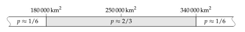
The true area is 243610 square kilometers. This area is comfortably in my predicted range and surprisingly close to the midpoint.

How surprising is the accuracy of the estimate?

The surprise can be quantified with a probability: the probability that the true value would be closer to the midpoint (the best estimate) than 243610 square kilometers is. Here, 243610 is 2.6 percent or a factor of 1.026 smaller than 250000. The probability that the true value would be within a factor of 1.026 (on either side) of the midpoint is the tiny shaded region of the log-normal distribution.

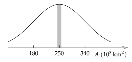
The region is almost exactly a rectangle, so its area is approximately its height multiplied by its width. The height is the peak height of a normal distribution. In \(\sigma\) = 1 units (in dimensionless form), this height is \(1/\sqrt{2 \pi}.\).

The width of the shaded region, also in \(\sigma = 1\) units, is the ratio

\[2 \times \frac{\textrm{dB equivalent for a factor of 1.026}}{\textrm{dB equivalent for a factor of 1.37}},\]

which is approximately 0.16. (The factor of 2 arises because the region extends equally on both sides of the peak.) Therefore, the shaded probability is approximately \(0.16/\sqrt{2 \pi}\) or only 0.07. I am surprised, but encouraged, by the accuracy of my estimate for the UK's land area. Once again, many individual errors--for example, in estimating journey times and speeds--have canceled out.

Exercise \(\PageIndex{1}\): Volume of a room

Estimate the volume of your favorite room, comparing your plausible ranges before and after using divide-and-conquer reasoning.

Exercise \(\PageIndex{2}\): Justifying the recipe for combining ranges

Use Bayes’ theorem to justify the recipe for combining plausible ranges

Exercise \(\PageIndex{3}\): Practice combining plausible ranges

You are trying to estimate the area of a rectangular field. Your plausible ranges for its width and length are 1…10 meters 10…100 meters, respectively.

a. What are the midpoints of the two plausible ranges?

b. What is the midpoint of the plausible range for the area?

c. What is the too-pessimistic range for the area, obtained by multiplying the corresponding endpoints?

d. What is the actual plausible range for the area, based on combining log-normal distributions? This range should be narrower than the pessimistic range in part (c)!

e. How do the results change if the ranges are instead 2…20 meters for the width and 20…200 meters for the length?

Exercise \(\PageIndex{4}\): Area of A4 paper

If you have a sheet of standard European (A4) paper handy, either in reality or mentally, find your plausible range for its area A by gut estimating its length and width (without using a ruler). Then compare your best estimate (the midpoint of your range) to the official area of An paper, which is 2⁻ⁿ square meters.

Exercise \(\PageIndex{5}\): Estimating a mass

In trying to estimate the mass of an object, your plausible range for its density is 1…5 grams per cubic centimeter and for its volume is 10…50 cubic centimeters. What is (roughly) your plausible range for its mass?

Exercise \(\PageIndex{6}\): Which is the wider range?

Suppose that your knowledge of the quantities a, b, and c is given by these plausible ranges:

a= 1…10

b = 1…10

c = 1…10.

Which quantity—abc or a²b—has the wider plausible range?

Exercise \(\PageIndex{7}\): Handling division

If a quantity a has the plausible range 1…4, and the quantity b has the plausible range 10…40, what are the plausible ranges for ab and for a/b?

7.2.2 Finding one-sigma endpoints before the midpoint

With our understanding of probability, we can explain two curious and seemingly arbitrary features of how we make gut estimates (Section 1.6). First, we learned not to ask our gut about its best estimate. Rather, we ask about its lower and upper endpoints, from which we find the best estimate as their midpoint. Second, in finding the endpoints, the standard we use is “mildly surprised”: We should be mildly surprised if the true value lies outside the endpoints. Quantitatively, “mild surprise” now means that the probability should 2/3 that the true value lies between the endpoints.

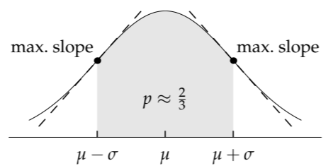
The first feature, that we estimate the endpoints rather than the midpoint directly, is explained by the shape of the log-normal distribution. Imagine trying to locate its midpoint by offering your gut candidate midpoints. The distribution is flat at the midpoint, so the probability hardly varies as the candidates change. Thus, your gut will answer with almost identical sensations of ease over a wide range around the midpoint. As a result, you cannot easily extract a decent midpoint estimate.

The solution to this problem explains the second curious feature: why the plausible range should enclose a probability of 2/3. The solution is to estimate the location of the steepest places on the curve. Those spots are the points of maximum slope (in absolute value). Around these values, the probability changes most rapidly and so does the sensation of ease.

If we use the most convenient logarithmic units, where the midpoint \(\mu\) is 0 and the half width \(\sigma\) is 1, then the log-normal distribution becomes the reasonably simple form

\[p(x) = \frac{1}{\sqrt{2 \pi}} e^{-x^{2}/2},\]

where x measures half widths away from the peak. Its slope p'(x) is a maximum where the derivative of p'(x), namely p"(x), is zero. These points are also called the inflection or zero-curvature points. (Where the curvature is zero, the curve is straight, so the dashed tangent lines pass through it.)

Ignoring dimensionless prefactors,

\[p'(x) \sim -xe^{-x^{2}/2}; \\ p"(x) \sim (x^{2} -1)e^{-x^{2}/2}.\]

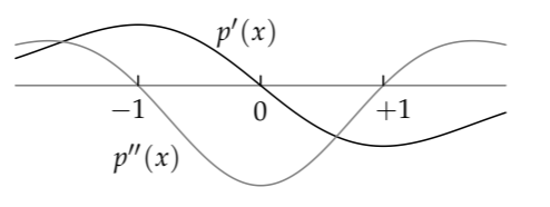
The second derivative is zero when x = ±1. This value is expressed in the \(\mu\) = 0, \(\sigma\) = 1 system of units. In the usual system, x = ±1 means the one-sigma points \(\mu \pm \sigma\). So the points of maximum (absolute) slope—the points that our gut can most accurately estimate—are the one-sigma points! We find them first and then find their midpoint.

When we estimate a 2/3-probability range, we are finding a one-sigma range almost exactly: In a normal or log-normal distribution, the one-sigma range contains approximately 68 percent of the probability, which is almost exactly 2/3. For comparison, the two-sigma range contains approximately 95 percent of the probability, which is a popular number in statistical analysis. Therefore, you may also want to find your two-sigma range (Problem 7.11). However, the slope at the two-sigma points is approximately a factor of 2.2 smaller than the slope at the one-sigma endpoints, so the two-sigma range is somewhat harder to estimate than is the one-sigma range. To find the two-sigma range, first estimate the one-sigma range, and then double its width (on a log scale).

This analysis of plausible ranges concludes our introduction to probability and the probabilistic basis of divide-and-conquer reasoning. We have learned that probabilities result from the incompleteness of our knowledge, and how acquiring knowledge changes our probabilities. In the next sections, we will use probability to master the complexity of systems with vast numbers of atoms and molecules, where complete knowledge would be impossible. The analysis begins with a special walk, the random walk.

Exercise \(\PageIndex{8}\): Two sigma range

My one-sigma range for the UK’s land area is 180 000…340 000 square kilometers. What is the two-sigma range?

Exercise \(\PageIndex{9}\): Gold or banknotes?

Having broken into a bank vault, do you take the banknotes or the gold? Assume that your capacity to carry loot is limited by mass rather than by volume.

a. Estimate gold’s value density (monetary value per mass)—for example, in dollars per gram. Give plausible ranges for your subestimates and find the resulting plausible range for the value density.

b. For your favorite banknote, give your plausible range for its value density and for the ratio

\[\frac{\textrm{value density of gold}}{\textrm{value density of the banknote}}.\]

c. Should you take the gold or the banknotes? Use a table of the normal distribution to evaluate the probability that your choice is correct.