8.2: Two regimes

After warming up with the examples in Section 8.1, let’s now look systematically at how to use the method of easy cases. The first step is to identify the dimensionless quantity. Once you know it—let’s call it \(\beta\)—the behavior of the system almost always divides into three regimes: \(\beta\) ≪ 1, \(\beta\) ∼ 1 (or \(\beta\) = 1), and \(\beta\) ≫ 1. In a common simplification, which is the subject of this section, one regime is impossible, so two regimes remain. (In Section 8.3, we will discuss what to do when all three regimes remain.) This simplification can happen because symmetry makes the bookend regimes \(\beta\) ≪ 1 and \(\beta\) ≫ 1 equivalent (Section 8.2.1) or because a geometric or physical constraint excludes one regime (Section 8.2.2).

8.2.1 Only two regimes because of symmetry

The bookend regimes \(\beta\) ≪ 1 and \(\beta\) ≫ 1 are often connected by a symmetry. Then the analysis at one bookend can be used as the analysis for the other bookend, and there are really two regimes: the symmetric bookends and the middle regime.

8.2.1.1 Why multiplication is more important than addition

As an example, here’s an easy-cases explanation of why, when estimating, multiplication is a more important operation than addition. Let’s say that we are estimating a cost, a force, or an energy consumption that splits into two pieces A and B to add together—for example, energy for heating and for transportation. Estimating A + B seems to require addition.

The need disappears after we examine the easy-cases regimes. The regimes are determined by a dimensionless quantity. Because A and B have the same dimensions, their ratio A/B is dimensionless, and it categorizes the three easy-cases regimes.

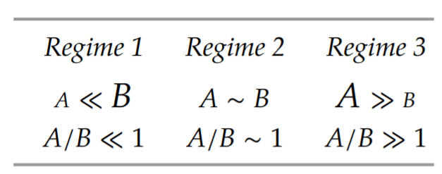
In the first regime, the sum A + B is approximately B. In the symmetric third regime, the sum is approximately A. The common feature of the first and third regimes—their invariant—is that one contribution dominates the other. Only the second regime, where A ∼ B is different. To handle it, just make the lumping approximation that A = B; then A + B ≈ 2A.

So, when estimating A + B, we do not need addition. In the first and third regimes, we just pick the larger contribution, A or B. In the second regime, we just multiply by 2.

8.2.1.2 Area of an ellipse

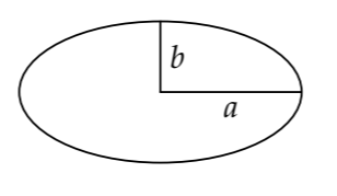
A mathematical example of this kind of symmetry happens when guessing the area of an ellipse. The dimensionless quantity is its aspect ratio a/b, where a is one-half of the horizontal diameter and b is one-half of the vertical diameter. Here are the regimes.

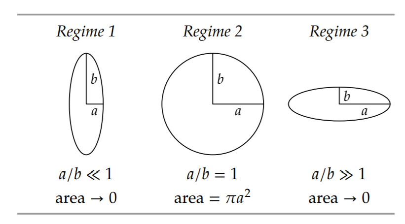
The first and third regimes are identical because of a symmetry: Interchanging a and b rotates the ellipse by 90^∘ (and reflects it through its vertical axis) without changing its area. Therefore, any proposed formula for the area must work in the first regime, must satisfy the symmetry requirement that interchanging a and b has no effect on the area (thereby taking care of the third regime), and must work for a circle (the second regime).

Because of the symmetry requirement, simple but asymmetric modifications of the area of a circle—namely, \(\pi a^{2}\) and \(\pi b^{2}\)—cannot be the area of an ellipse. A plausible, symmetric alternative is \(\pi (a^{2} + b^{2})/2\). In the second regime, where \(a=b\), it correctly predicts the area of a circle. However, it fails in the first regime: The area isn’t zero even when a = 0.

Is there an alternative that passes all three tests?

A successful alternative is \(\pi a b\). It predicts zero area when a = 0; it is symmetric; and it works when a = b. It is also the correct area.

8.2.1.3 Atwood machine

In the preceding examples, we had a ready-made dimensionless group and used it to categorize the three easy-cases regimes. The next example shows what you do when there is no group handy: Use dimensional analysis to make one. Then use the group to categorize the regimes and understand the system’s behavior. Easy cases and dimensional analysis work together.

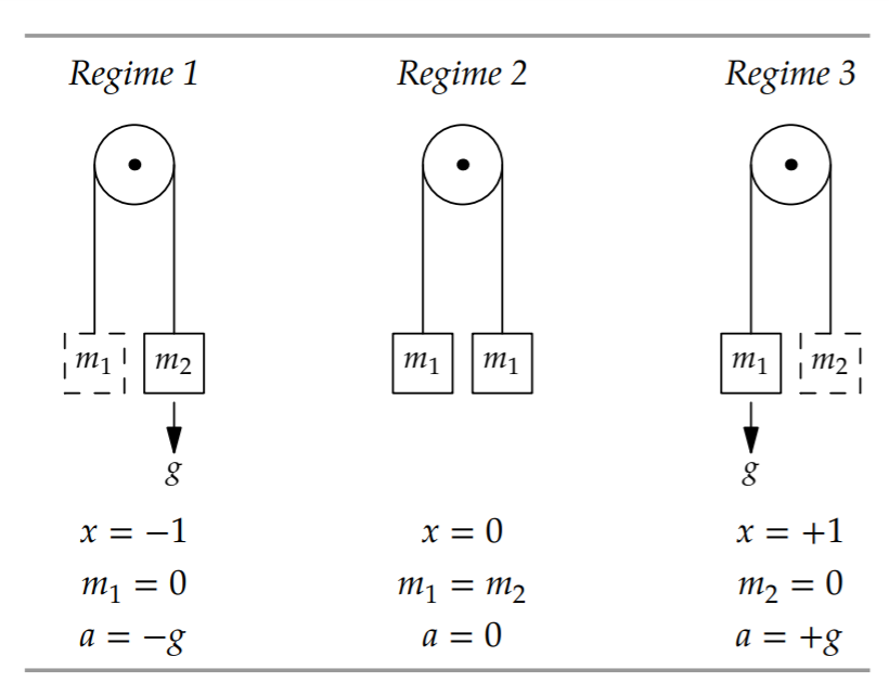
The example is the Atwood machine, a staple of the introductory mechanics curriculum. Two masses, m₁ and m₂, are connected by a massless, frictionless string and are free to move up and down because of the pulley. This machine, invented by the Reverend George Atwood, reduces the effective gravitational acceleration by a known fraction and makes constant-acceleration motion easier to study. (A historical discussion of the Atwood machine is given by Thomas Greenslade in [27].) Today its principle is used in elevators: The elevator car is m₁, and the counter weight is m₂.

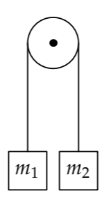
What is the acceleration of the masses?

Our second step is to identify the easy-cases regimes, but our first step is to find the dimensionless group that categorizes them. Therefore, we make our list of relevant quantities and their dimensions. The goal is the acceleration of the masses. Because they are connected by a string, their accelerations have the same magnitude but opposite directions. Let a be the downward acceleration of the mass on the left—whether it is labeled m₁ or m₂ (planning for an application of symmetry). Because a is our goal quantity, it is the first quantity on the list. The motion is caused by gravity, so the list includes g. Finally, the masses affect the acceleration, so the list includes m₁ and m₂. And that’s the whole list.

a	LT^-2	acceleration
g	LT^-2	gravity
m1	M	left block's mass
m2	M	right block's mass

Doesn’t the tension also affect the acceleration?

The tension has an important effect: Without the tension, there would be no problem to solve, because each mass would accelerate downward at g. However, the tension is a consequence of m₁, m₂, and g—quantities already on the list. Thus, tension is redundant; adding it would only confuse the dimensional analysis.

This list contains only two independent dimensions: mass (M) and acceleration (LT⁻²). Four quantities built from two independent dimensions produce two independent dimensionless groups. The most natural choices are the acceleration ratio a/g and the mass ratio m₁/m₂. Then the most general dimensionless statement is

\[\frac{a}{g} = f (\frac{m_{1}}{m_{2}}),\]

where \(f\) is a dimensionless function.

Although the next step is to use easy cases to guess the dimensionless function, first pause for a moment. The more we think now in order to choose a suitable representation, the less algebra we have to do later. Here, the ratio m₁/m₂ does not respect the symmetry of the problem. Interchanging the masses m₁ and m₂ turns m₁/m₂ into its reciprocal: It raises the ratio to the −1 power. Meanwhile, because the left mass is now m₂, which has the opposite acceleration to m₁, this symmetry operation changes the sign of the acceleration a (which measures the downward acceleration of the left mass): It multiplies the acceleration by −1. The function \(f\) will have to incorporate this change in the nature of the symmetry and will have to work hard to turn m₁/m₂ into an acceleration. Therefore, \(f\) will be complicated and hard to guess. (You can find it anyway in Problem 8.3.)

A more symmetric alternative to the ratio m₁/m₂ is the difference m₁ − m₂. Now interchanging m₁ and m₂ negates m₁ − m₂, just as it negates the acceleration. Unfortunately, m₁ − m₂ is not dimensionless! It has dimensions of mass. To make it dimensionless, we need to divide it by another mass, say m₁, to make (m₁−m₂)/m₁. Unfortunately, that choice abandons our beloved symmetry. Dividing instead by the symmetric combination m₁ + m₂ solves all the problems. Let’s call the result x:

\[x \equiv \frac{m_{1} - m_{2}}{m_{1} + m_{2}}.\]

This ratio is dimensionless and respects the problem’s symmetry. With it as the dimensionless group, the most general dimensionless statement is

\[\frac{a}{g} = h(\frac{m_{1} - m_{2}}{m_{1}+m_{2}}),\]

where ℎ is a dimensionless function (different from \(f\) ). (This combination of m₁ and m₂ doesn’t satisfy the definition of a group given in Section 5.1.1, as a dimensionless product of the quantities raised to various powers. However, it is worth extending the concept to include such combinations.)

To guess ℎ, study the easy-cases regimes according to x. They are three: x = −1 (imagine that m₁ = 0), x = 0 (when m₁ = m₂), and x = +1 (imagine that m₂ = 0). Here you see how easy cases help us. The extremity of the first and third regimes and the simplicity of the second regime amplify our physical intuition and help our gut predict the behavior.

In the first regime, m₂ falls as if there were no mass on the other end of the string. Thus, m₁ rises with acceleration +g. Because a measures the downward acceleration of the left mass, a = −g. In the third, symmetric regime, m₁ accelerates downward as if there were no mass on the other end, so a = +g. In the second regime, where x = 0 or m₁ = m₂, the masses are in equilibrium, and a = 0.

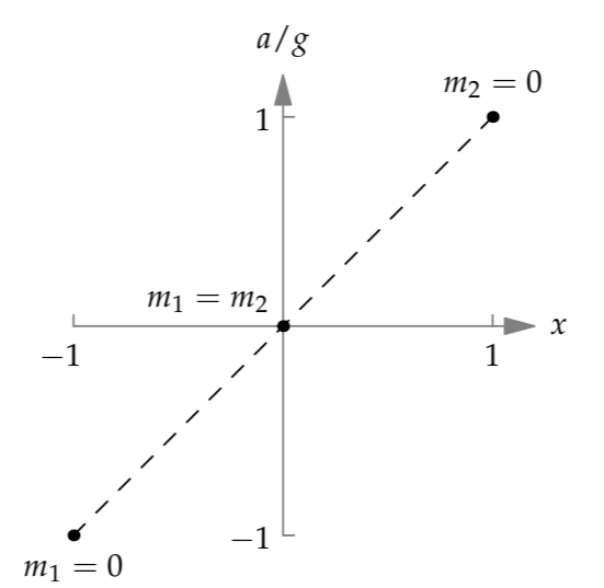
Here are the three easy cases plotted on a graph of the dimensionless acceleration a/g versus the dimensionless mass parameter x. Based on this graph, the simplest conjecture, an educated guess, is that the full graph of ℎ(x) is the straight line of unit slope passing through the three points. Thus, its equation is a/g = x. In terms of the masses, the equation is

\[\frac{a}{g} = \frac{m_{1} - m_{2}}{m_{1} + m_{2}}.\]

In Problem 8.4(d), you solve for the acceleration by using Newton’s laws to find the tension in the string. Then you’ll confirm our reasonable conjecture based on easy-cases reasoning.

Exercise \(\PageIndex{1}\): Using the less symmetric dimensionless group

Find the dimensionless function \(f\) based on the simpler, but less symmetric, dimensionless group \(m_{1}/m_{2}\):

\[\frac{a}{g} = f(\frac{m_{1}}{m_{2}}).\]

Compare it to the dimensionless function that results from choosing the symmetric form \((m_{1}-m_{2})/(m_{1} + m_{2})\) as the independent variable.

Exercise \(\PageIndex{2}\): Tension in the string in Atwood's machine

In this problem you use easy cases to guess the tension in the connecting string.

a. The tension T, like the acceleration, depends on m₁, m₂, and g. Explain why these four quantities produce two independent dimensionless groups.

b. Choose two suitable independent dimensionless groups so that you can write an equation for the tension in this form:

\[\textrm{group proportional to } T = f(\textrm{(group without } T \textrm{).}\]

c. Use easy cases to guess \(f\) ; then sketch \(f\).

d. Solve for T using freebody diagrams and Newton’s laws. Then compare that result with your guess in part (c), and use T to find a, the downward acceleration of m₁.

8.2.2 Only two regimes because of a restriction

In the preceding examples, there were three regimes of a dimensionless quantity, but the two bookend regimes were connected by a symmetry operation and were therefore the same situation. Therefore, there were only two qualitatively different regimes. In the next group of examples, there are only two regimes for a different reason: A geometric or physical constraint excludes one bookend regime.

8.2.2.1 Projectile range

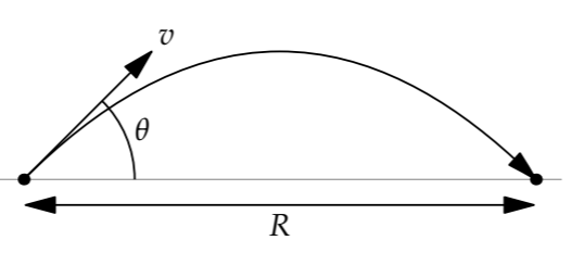
In Section 4.2.3, we used proportional reasoning to show that the range of a projectile should have the form \(R \sim v^{2}/g\), where \(v\) is its launch velocity. However, we didn’t determine how the launch angle \(\theta\) affects the range. We can do so using easy cases, with help from dimensional analysis.

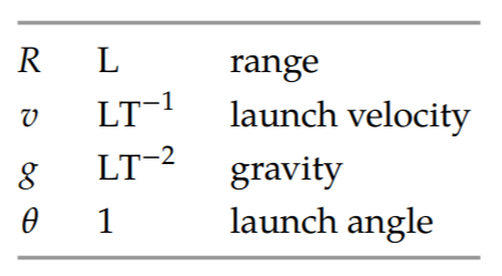
Now the problem contains four quantities: R, \(v\), g, and \(\theta\). Four quantities containing two independent dimensions (for example, L and T) produce two independent dimensionless groups. A reasonable pair is the launch angle \(\theta\)—which is already dimensionless—and, based on the proportional-reasoning result, \(Rg/v^{2}\). Then the most general dimensionless statement is

\[\frac{Rg}{v^{2}}= f(\theta),\]

where \(f\) is a dimensionless function. Solving for R,

\[R = \frac{v^{2}}{g} \times f(\theta).\]

Dimensional analysis does not tell us the form of \(f\), but we can guess it by examining the easy cases. Easy-cases reasoning is a way of introducing physical knowledge.

Because angles are dimensionless, \(\theta\) can categorize the easy-cases regimes. The natural easy cases of any quantity are its extremes: \(\theta\) ≪ 1 (our usual first regime) and \(\theta\) ≫ 1 (our usual third regime). The regime \(\theta\) ≪ 1 includes the smallest launch angle \(\theta\) = 0^∘. Then the range is zero: The projectile starts at ground level, is launched horizontally, and hits the ground immediately. However, the opposite extreme \(\theta\) ≫ 1 is not useful, because angles are periodic. Any angle beyond 2\(\pi\) is already handled by an angle less than 2\(\pi\). Our usual third regime is therefore geometrically excluded.

Our usual second regime is \(\theta\) ∼ 1. Here, the easy angle comparable to 1 (in radians) is \(\theta\) = 90^∘ (\(\pi\)/2 radians). This angle describes a vertical launch, which doesn’t produce any range. Thus, R in this regime is also 0.

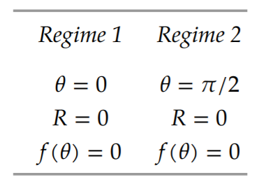
The two regimes are therefore \(\theta\) = 0 (an example of \(\theta\) ≪ 1) and \(\theta\) = \(\pi\)/2 (an example of \(\theta\) ∼ 1).

What reasonable functions satisfy the two easy-cases constraints on \(f(\theta)\)?

One such function is the product of two straight lines, each line ensuring that one of the constraints is satisfied:

\[f(\theta) = \theta (\frac{\pi}{2} - \theta).\]

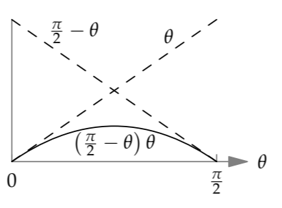
However, this functional form looks funny. The \(\pi\)/2 in the second factor appears by magic, with no obvious origin in the equations of free fall. Worse, the guess is not periodic. Increasing \(\theta\) by 2\(\pi\) shouldn’t change the range, but it changes this proposed \(f\). Thus we need to keep looking.

A similar but less magical form, also the product of two factors, is

\[f(\theta) \sim sin \theta cos \theta.\]

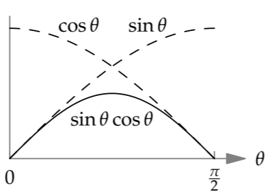
The cos \(\theta\) factor ensures that \(f (\pi/2) = 0\). The sin \(\theta\) factor ensures that \(f(0) = 0\). This functional form is also periodic. And it has a physical justification: sin \(\theta\) is the trigonometric factor that converts the launch velocity \(v\) into its vertical component \(v_{y}\); the cos \(theta\) factor does the same for the horizontal component \(v_{x}\). Because these velocities appeared in the proportional-reasoning analysis of Section 4.2.3, we already know that they are physically relevant, making this functional form more plausible than the preceding form.

The resulting range, including the effect of the angle, is then

\[R \sim \frac{v^{2}}{g} sin \theta cos \theta.\]

This form is correct, and the dimensionless prefactor turns out to be 2 (as you can show in Problem 8.5).

Exercise \(\PageIndex{3}\): Finding the dimensionsless constant

Extend the proportional-reasoning analysis of Section 4.2.3 to show that the missing dimensionless prefactor in the projectile range is 2.

8.2.2.2 Light bending with large angles

Our next example of a physical limit excluding a third regime also involves an angle: the bending of light by gravity.

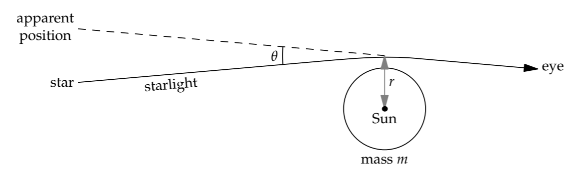
In Section 6.4.6, we used lumping to find that the gravitational field from a mass m bends light by an angle

\[\theta \sim \frac{Gm}{rc^{2}},\]

where r is the distance of closest approach.

This angle is dimensionless. Thus, let’s use it to categorize and to investigate the easy cases of light bending. The first regime is \(\theta\) ≪ 1—for example, the Sun bending starlight by roughly 1 arcsecond. The second regime is \(\theta\) ∼ 1. In this regime, a new physical phenomenon appears, and lumping will help us analyze it.

The lumping analysis is based on the American television cartoon of the Road Runner pursued by the Wile E. Coyote. The road runner runs across a chasm, followed by the coyote. They cruise as if gravity is gone, until the road runner, safely across the gap, holds up a sign with an arrow pointing downward explaining, “Gravity this way.” The coyote looks down, remembers the existence of gravity, and falls into the chasm.

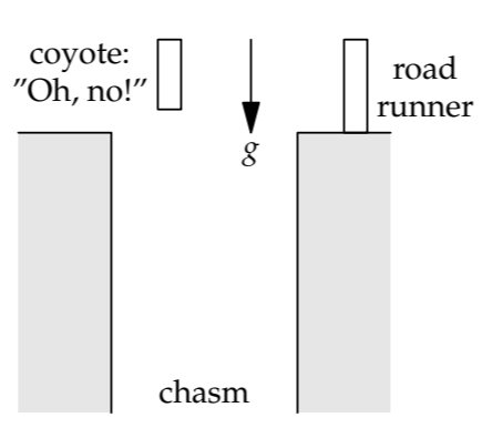
In the coyote model, light zooms past the mass (say, a star) ignorant of gravity. After it has gone too far—by a distance comparable to r—the star holds up a sign saying, “You forgot about gravity! Please bend by \(\theta\) now!” In this second regime, \(\theta\) ∼ 1. The following pictures and analysis are clearest if \(\theta = \pi/2\) (or 90^∘), so let’s use 90^∘ to represent the \(\theta\) ∼ 1 regime.

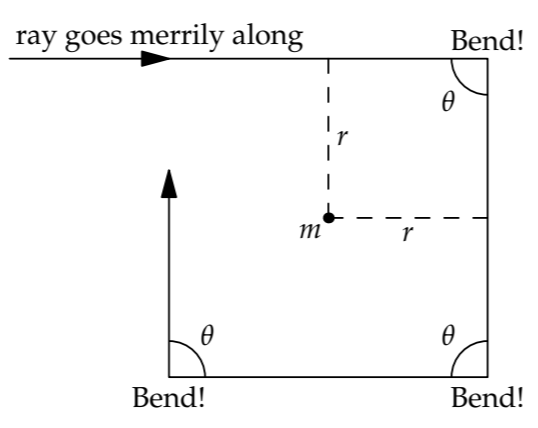
The ray, on command, bends by 90^∘. It travels along and gets reminded again. The distance of closest approach is still r, so \(\theta\) is still 90^∘. The beam traces out a square. Although the ray doesn’t actually follow this path with its sharp corners, the path illustrates the fundamental feature of the \(\theta\) ∼ 1 regime: The ray is in orbit around the star. When \(\theta\) ∼ 1, light gets captured by the strong gravitational field. The third regime, \(\theta\) ≫ 1, doesn’t introduce a new physical phenomenon—the light is still captured by the gravitational field. In either regime, the mass is a black hole.

Exercise \(\PageIndex{4}\): Guessing a variance

The variance is a squared measure of the spread in a distribution:

\[\textrm{Var} x = \langle x^{2} \rangle - \langle x \rangle ^{2}.\]

where \(\langle x^{2} \rangle\) is the average or expected value of x² (the mean square) and \(\langle x \rangle\) is the average value of x (the mean).

a. Use an easy case to convince yourself that the mean square \(\langle x^{2} \rangle\) is never smaller than the squared mean \(\langle x \rangle ^{2}\).

b. The simplest possible distribution has only two possibilities, x = 0 and x = 1, with probabilities 1 − p and p, respectively. This distribution describes a coin toss where heads (represented by x = 1) comes up with probability p. Use easy cases to guess Var x

Exercise \(\PageIndex{5}\): Local black hole

What is roughly the largest radius that the Earth could have, with its current mass, and be a black hole?