8.3: Three Regimes

Two regimes are easier than three. Therefore, we studied that case first to develop experience and identify the transferable ideas. Fortunately, even when a complex situation has three regimes, two simplifications are possible. First, the bookend regimes are often easier than the middle regime (Section 8.3.1). Then we study the bookends and, to predict the behavior in the middle, interpolate between the bookends. Alternatively, two effects compete and reach a draw in the middle regime (Section 8.3.2). This middle regime is then the regime found in nature.

8.3.1 Three regimes where the bookends are easier

In a common easy-cases situation, the dimensionless number categorizing the three regimes is a ratio between two physical effects. Then the two bookends are the easiest regimes to analyze—because at each bookend, one or the other effect vanishes. We’ll practice this analysis in an example from introductory mechanics (Section 8.3.1.1); then we’ll graduate to drag (Section 8.3.1.2).

8.3.1.1 Rolling down the plane

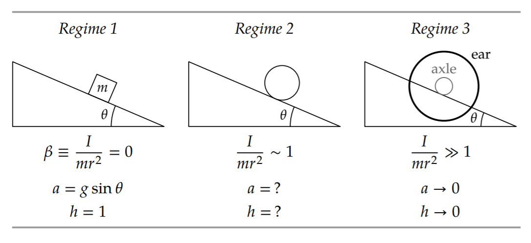
As our introductory example, let’s revisit objects rolling without slipping down an inclined plane. The goal will be to predict an object’s acceleration a along the plane. Dimensional analysis, from Problem 5.18, tells us that the most general dimensionless statement about a is where \(f\) is a dimensionless function, \(\theta\) is the incline angle, I is the object’s moment of inertia, m is its mass, and r is its radius. The only quantities that affect the acceleration are the two dimensionless groups: the incline angle \(\theta\) and the dimensionless mass distribution \(I/mr^{2}\). The ratio \(I/mr^{2}\), and therefore the acceleration, is invariant under changes to the object’s mass or radius (for example, making a bigger ring or disc). In plainer language, which however doesn’t connect as much to symmetry reasoning, simply changing the object’s mass or radius without changing its shape does not change its acceleration.

\[\frac{a}{g} = f (\theta, \frac{I}{mr^{2}}),\]

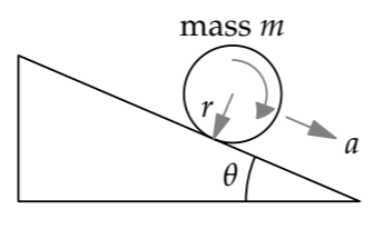
Which shape rolls faster—a ring or a disc?

In this comparison, the inclined plane and thus the incline angle \(\theta\) remain fixed. However, the dimensionless group \(I/mr^{2}\) changes and can categorize the easy-cases regimes. This group occurs repeatedly in the analysis, so we’ll often symbolize it as \(\beta\). By understanding the behavior in the regimes defined by \(\beta\), we’ll be able to predict the result of the ring–disc race.

Let’s start with the first regime, \(I/mr^{2} =0\). This regime is reached by making I zero. Then rolling, represented by I, becomes irrelevant. The object moves as if it were sliding down the plane without friction. Its acceleration is then \(g sin \theta\), and \(a/g = sin \theta\).

With this easy-cases result, we can simplify the unknown function \(f\), which unfortunately is a function of two dimensionless groups. As a reasonable conjecture, the dependence on angle is probably still sin \(\theta\), even when I is not zero. Then the dimensionless statement simplifies to

\[\frac{a}{g} = h (\frac{I}{mr^{2}}) sin \theta,\]

where ℎ is a dimensionless function of only one group.

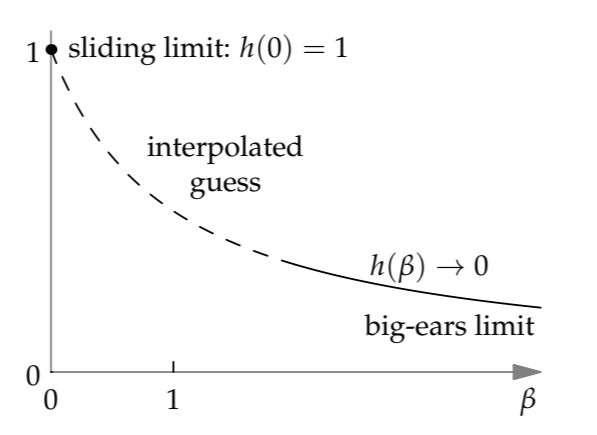
Let’s guess h using easy cases of \(\beta = I/mr^{2}\). The three regimes will be \(\beta\) = 0 (a special case of \(\beta\) ≪ 1), \(\beta\) ∼ 1, and \(\beta\) ≫ 1. In the first regime, when \(\beta\) = 0, rolling is unimportant, as we just observed. Therefore, \(a/g = sin \theta\) and the dimensionless function ℎ(\(\beta\)) is just 1.

The middle regime \(\beta\) ∼ 1 is difficult to analyze without a full calculation. Yet the goal of an easy-cases analysis is to make the situation simple enough that the behavior is easy to see and we can skip the full calculation. Even the simplest value within this regime, \(\beta\) = 1, is not any easier than other values. (It describes the ring, where all mass is distributed at the edge of the object, at a distance r from the center). The middle regime is, as promised, the difficult regime. Neither fish nor fowl, it mixes rolling and sliding in comparable amounts.

The solution is to study the third regime, where \(\beta\) ≫ 1, and then to interpolate between the first and third regimes in order to predict the behavior in the middle regime. (We implicitly used this interpolation approach in Section 6.4.3, when we estimated the time and distance for a falling cone to reach its terminal speed.)

For an object rolling down the plane, how can \(\beta\) be increased beyond 1?

There seems to be no way to increase \(\beta\) beyond 1: When \(\beta\) = 1, all mass is already distributed at the edge. Fortunately, the subtle point is that, in the dimensional analysis, r is the rolling radius, rather than the radius of the object, because the rolling radius determines the torque and the motion. The object’s radius can be larger than the rolling radius. This possibility allows us to increase \(\beta\) as much as we want.

As an example, imagine a barbell used for weight lifting: A thin axle of radius r connects two large and massive ears of radii R. Place the axle on the inclined plane, with the ears beyond the plane. The rolling radius is the radius r of the axle. However, the moment of inertia I is mostly due to the large ears, because

\[\textrm{moment of inertia} \propto (\textrm{distance from the axis rotation})^{2}.\]

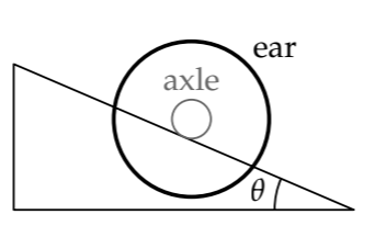
Thus, \(I \sim mR^{2}\), where m is the combined mass of the two ears, which is almost the same as the mass of the whole object. By choosing R ≫ r, we can make \(\beta\) ≫ 1:

\[\beta \equiv \frac{I}{mr^{2}} \sim (\frac{R}{r})^{2} >> 1.\]

How quickly does this large-\(\beta\) object accelerate down the plane?

This extreme regime is easier to think about than the intermediate regime \(\beta\) = 1. The extremity of the \(\beta\) ≫ 1 regime amplifies our intuition and shouts loudly enough for our gut to hear. Then our gut’s answer is loud enough for us to hear: The barbell, rolling on its small axle, as long as it doesn’t slip, will creep down the plane (the italics represent my gut’s shouting). Going fast would, in spinning up the ears, demand far more energy than gravity can provide. Thus, as the ears get ever larger and \(\beta\) goes to infinity, the dimensionless rolling factor ℎ(\(\beta\)) goes to zero.

A simple guess that accounts for the two extreme regimes is

\[h(\beta) = \frac{1}{1 + \beta}.\]

In terms of the original quantities, the acceleration would be

\[a = \frac{g sin \theta}{1 + I/mr^{2}}.\]

This educated guess turns out to be correct (Problem 8.8). Now we can answer our original question about which shape rolls faster. The farther outward the mass is distributed, the greater \(\beta\) is, so \(\beta_{ring} > \beta_{disc}\). Because a decreases as \(\beta\) increases, the disc rolls faster than the ring.

Exercise \(\PageIndex{1}\): Exact solution to rolling down the plane

Use conservation of energy to find the acceleration of the object along the plane, and confirm the guess based on the easy-cases regimes.

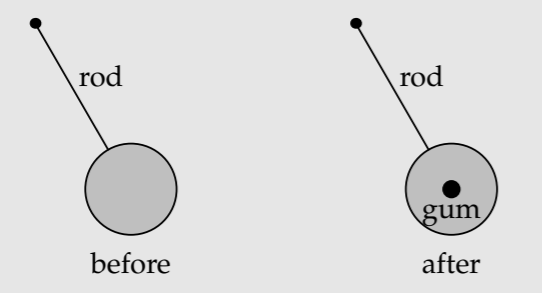
Exercise \(\PageIndex{2}\): A pendulum with chewing gum

A pendulum with a disc as the pendulum bob is oscillating with period T. You then stick a small piece of chewing gum onto the center of the disc. How does the gum affect the pendulum’s period: an increase, no effect, or a decrease?

8.3.1.2 Drag using easy cases

Drag, like any phenomenon related to fluids, is a hard problem. In particular, there is no way to calculate the drag coefficient c_d as a function of Reynolds number Re—even for simple shapes such as a sphere or a cylinder. However, dimensional analysis (Section 5.3.2) has told us that

\[\underbrace{\textrm{drag coefficient}}_{c_{d}} = f\underbrace{(\textrm{Reynold's number})}_{\textrm{Re}}.\]

However, dimensional analysis could not tell us the function \(f\). That’s no slur on dimensional analysis; finding the whole function is beyond our present-day understanding of mathematics. However, we can understand much about \(f\) in two easy cases: the bookend regimes Re ≫ 1 and Re ≪ 1. In the difficult middle regime Re ∼ 1, the function \(f\) interpolates between its behavior in the two extremes.

Low Reynolds number. Flows at low Reynolds number, although not as frequent in everyday experience as flows at high Reynolds number, include a fog droplet falling in air (Problem 8.13), a bacterium swimming in water (discussed in the classic paper “Life at low Reynolds number” [39]), and ions conducting electricity in seawater (Problem 8.10). Our goal here is to find the drag coefficient in the regime Re ≪ 1.

The Reynolds number (based on radius) is \(vr/\nu\), where \(v\) is the speed, \(r\) is the object’s radius, and \(\nu\) is the kinematic viscosity of the fluid. Therefore, to shrink Re, either make the object small, make the object’s speed low, or use a fluid with high viscosity. The method does not matter, as long as Re is small: The drag coefficient is determined not by any of the individual parameters \(r\), \(v\), or \(\nu\), but rather by the abstraction Re. We’ll choose the means that leads to the most transparent physical reasoning: making the viscosity huge. Imagine, for example, a tiny bead oozing through a jar of cold honey. (The tininess of the bead further reduces Re.)

In this extremely viscous flow, the drag force, as you might expect, is produced directly by viscous forces. As you reasoned in Problem 7.25, viscous forces, which are proportional to the kinematic viscosity \(nu\), are given by

\[F_{viscous} \sim \rho \nu \times \textrm{velocity gradient} \times \textrm{area}.\]

The area is the surface area of the object. The velocity gradient is the rate at which velocity changes with distance; it is analogous to the concentration gradient \(\Delta n/ \Delta x\) in the Fick’s-law analysis of Section 7.4.2 or to the temperature gradient \(\Delta T/ \Delta x\) in the heat-flow analysis of Section 7.4.4.

Because the drag force is due to viscous forces directly, it should be proportional to \(\nu\). This constraint determines the form of the function \(f\) and therefore the drag force. Let’s write out the dimensional-analysis result connecting the drag coefficient and the Reynolds number:

\[c_{d} \equiv \frac{F_{d}}{\frac{1}{2} \rho A_{cs} v^{2}} = f \underbrace{(\frac{vr}{\nu})}_{\textrm{Re}},\]

where F_d is the drag force and A_cs is the object’s cross-sectional area. In terms of the radius, \(A_{cs} \sim r^{2}\), so

\[\underbrace{\frac{F_{d}}{\rho r^{2} v^{2}}}_{\sim c_{d}} \sim f \underbrace{(\frac{vr}{\nu})}_{\textrm{Re}}.\]

The viscosity \(\nu\) appears only in the Reynolds number, where it appears in the denominator. To make F_d proportional to \(\nu\) requires making the drag coefficient proportional to 1/Re. Equivalently, the function \(f\), when Re ≪ 1, is given by \(f(x) \sim 1/x\). Then

\[\frac{F_{d}}{\rho r^{2} v^{2}} \sim \frac{\nu}{vr}.\]

For the drag force itself, the consequence is (as you found in Problem 7.26)

\[F_{d} \sim \rho r^{2} v^{2} \frac{\nu}{vr} = \rho \nu v r.\)

This result is valid for almost all shapes; only the dimensionless prefactor changes. For a sphere, the British mathematician George Stokes showed that the missing dimensionless prefactor is \(6 \pi\):

\[F_{d} = 6 \pi \rho \nu v r.\]

Accordingly, this result is called Stokes drag.

High Reynolds number. Because the Reynolds number \(rv/\nu\) contains three quantities, the limit of high Reynolds number can also be reached in three ways, all of which produce the same behavior. We’ll choose the method that is easiest to feel, which is to shrink the viscosity \(\nu\) to 0. In this limit, called form drag, viscosity disappears from the problem and the drag force should not depend on viscosity. This reasoning contains several untruths, but they are subtle and the conclusion is mostly correct. (Clarifying the subtleties required centuries of progress in mathematics, culminating in the theory of singular perturbations and boundary layers, the subject of Section 7.3.4 and discussed much more in Physical Fluid Dynamics [46].)

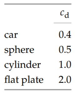
Without viscosity and thus without the Reynolds number to depend on, the dimensionless function \(f\) must be a constant! Its value depends on the shape of the object and typically ranges from 0.5 to 2 Because the drag coefficient is \(F_{d}/\frac{1}{2} \rho v^{2} A_{cs}\), the drag force is

\[F_{d} \sim \rho v^{2} A_{cs}.\]

This result agrees with our analysis in Section 3.5.1 based on energy conservation. In that analysis, we had implicitly assumed a high Reynolds number without knowing it.

Exercise \(\PageIndex{3}\): Conductivity of seawater

Estimate the conductivity of seawater by assuming that the current-carrying ions (Na⁺ or Cl⁻) travel with a shell one layer thick of water molecules around them.

Exercise \(\PageIndex{4}\): Drag coefficient resulting from Stokes drag

At low Reynolds number, the drag force on a sphere is \(F = 6 \pi \rho \nu v r\) (Stokes drag). Find the drag coefficient c_d as a function of Reynolds number, basing the Reynolds number on the sphere’s diameter rather than its radius.

Exercise \(\PageIndex{5}\): Choosing the high- or low-Reynolds-number regime

To estimate the terminal speed of a raindrop (Problem 3.37), you implicitly used the high-Reynolds-number regime. Now that you know another regime, how can you choose which regime to use? Without knowing which regime, you cannot find the terminal speed. Without the terminal speed, how do you find Reynolds number, which you need to choose the regime? The answer is to choose a regime and see whether the result is self-consistent. If it is not, choose the other regime.

As practice with this reasoning, assume that the Reynolds number for the falling raindrop is small and therefore that the drag force F_d is given by Stokes drag:

\[F_{d} \sim \rho_{air} \nu vr.\]

Estimate the resulting terminal speed \(v\) for the raindrop (diameter of about 0.5 centimeters). Then check the assumption that Re≪ 1.

Exercise \(\PageIndex{6}\): Terminal speed of fog droplets

1. Estimate the terminal speed of fog droplets (\(r \sim 10 \mu m\)). In estimating the drag force, use either the limit of low or high Reynolds numbers—whichever limit you guess is more likely to be valid. (Problem 8.12 introduces this reasoning.)
2. Use the speed to estimate the Reynolds number and check whether you used the correct limit for the drag force. If not, try the other limit!
3. Fog is a low-lying cloud. How long does a fog droplet require to fall 1 kilometer (a typical cloud height)? What is the everyday effect of this settling time?

Interpolation. We now know the drag force in the two extreme regimes: viscous drag (low Reynolds number) and form drag (high Reynolds number). Interpolating between these regimes is easiest in dimensionless form—that is, in terms of the drag coefficient rather than the drag force

When Re ≫ 1, the drag coefficient c_d is roughly 0.5 (for a sphere). On log–log axes, the Re ≫ 1 behavior is a straight line with zero slope. In the Re ≪ 1 regime, you should have found in Problem 8.11 that the drag coefficient (for a sphere) is 24/Re, where the Reynolds number is based on the diameter rather than the radius: The 1/Re scaling happens because, as we just deduced, \(f(\textrm{Re}) \sim 1/\textrm{Re}\) to make the drag force proportional to viscosity \(\nu\); the dimensionless prefactor of 24 is what you had to compute. On log–log axes, the Re ≪ 1 behavior is also a straight line but with a −1 slope.

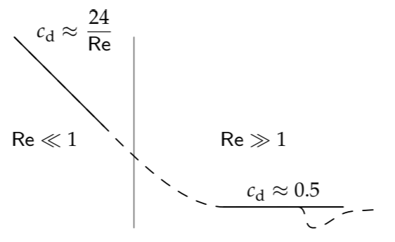
The dashed line interpolates between the extremes. The final twist is that at Re ∼ 3 × 10⁵, the boundary layer becomes turbulent (Problem 7.23), and the drag coefficient drops significantly. With that caveat, we have explained the main features of drag, a ubiquitous force in the living world.

Exercise \(\PageIndex{7}\): Q as an easy-cases parameter

A damped spring–mass system has a dimensionless measure of damping known as the quality factor Q, which you studied in Problem 5.53. Choose Q ≪ 0.5, Q = 0.5, or Q ≫ 0.5 to describe each of the three regimes: (a) underdamped, (b) critically damped, and (c) overdamped

Exercise \(\PageIndex{8}\): Floating on water

Some insects can float on water thanks to the surface tension of water. Extend the analysis of this effect from Problem 5.52 by estimating the dimensionless ratio

\[R \equiv \frac{\textrm{force due to surface tension}}{\textrm{weight of the bug}}\]

as a function of the bug’s size l (as a length). Interpret the regimes R ≪ 1 and R ≫ 1, and find the critical bug size l₀ for floating on water

Exercise \(\PageIndex{9}\): Energy loss in highway versus city driving

Explain why the following dimensionless ratio measures the importance of drag:

\[\frac{\textrm{mass of fluid swept out}}{\textrm{mass of object}}.\]

An equivalent computation, except for a dimensionless factor of order unity, is

\[\frac{\textrm{fluid density}}{\textrm{object density}} \times \frac{\textrm{distance traveled}}{\textrm{size of object}}\]

where the size of the object is its linear dimension in the direction of travel. When this ratio is comparable to unity, drag significantly affects the trajectory.

Apply either form of the ratio to a car during city driving, and find the distance d at which the ratio becomes significant (say, roughly 1). How does the distance compare with the distance between stop signs ortraffic lights on city streets? What therefore is the main mechanism of energy loss in city driving? How does this analysis change for highway driving?

Exercise \(\PageIndex{10}\): Gain of an RC circuit

The low-pass RC circuit of Section 2.4.4 is amenable to easy-cases analysis. With the abstraction of capacitive impedance (Section 2.4.4), explain the unity gain at low frequency and why the gain goes to zero at high frequency. What is the dimensionless way to say “high frequency”?

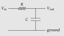
Exercise \(\PageIndex{11}\): Bode magnitude sketch for an RC circuit

A Bode magnitude plot is a log–log plot of ∣gain∣ versus frequency. In a lumped Bode sketch, which often gives the most insight into the behavior of a system, the segments of the plot are straight lines. Make the Bode magnitude sketch for the low-pass RC circuit of Problem 8.17, labeling the slopes and intersection points.

8.3.2 Three regimes where two effects compete

In the final group of three-regime examples, the three regimes are again based on the relative size of two physical effects. However, in contrast to the examples in Section 8.3.1, where we chose a regime—for example, by choosing a flow speed and thus the Reynolds number—here nature chooses. Nature chooses the middle regime, where the two competing physical effects reach a draw. The method of easy cases shows how that choice is made.

8.3.2.1 Height of the atmosphere

Competition between physical effects is the theme of the wonderful Gases, Liquids and Solids and Other States of Matter [43, pp. xiii], where we learn how “the three primary states of matter are the result of competition between thermal energy and intermolecular forces.” The following example, estimating the height of our atmosphere, illustrates an analogous competition: between thermal energy and gravity. Here is how these two physical effects determine the height of the atmosphere.

1. Thermal energy. Thermal energy gives the molecules speed. Unfettered by gravity, the air molecules and the atmosphere would disperse into space. Thermal energy is therefore responsible for increasing the atmosphere’s height.
2. Gravity. Gravity pulls air molecules downward. If gravity is the only effect, meaning that thermal motion is absent (the atmosphere is at absolute zero), then gravity pulls the molecules all the way to the ground. Gravity therefore decreases the atmosphere’s height.

A dimensionless measure of the relative size of the two effects is a comparison of the typical gravitational energy with the thermal energy of one molecule. The typical thermal energy is k_BT. With m for the molecule’s mass and H for the characteristic or typical or scale height of the atmosphere, the typical gravitational potential energy is mgH. The energy ratio is then

\[\beta \equiv \frac{mgH}{k_{B}T}.\]

This ratio categorizes the three easy-cases regimes: \(\beta\) ≪ 1, \(\beta\) ∼ 1, and \(\beta\) ≫ 1.

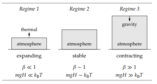
In the first regime, the atmosphere is expanding: The molecules have so much thermal energy that they escape farther from Earth. In the third regime, the atmosphere is contracting: The molecules do not have enough thermal energy to resist gravity as it pulls them back to Earth. The happy medium, where the atmosphere is stable, is the middle regime.

Therefore, the regime is chosen not by us but by nature. The height of the atmosphere is determined by the requirement that the two effects compete and reach a draw—when the two effects are comparable in strength. In that regime, \(mgH \sim k_{B}T\), so the atmosphere’s scale height is

\[H \sim \frac{k_{B}T}{mg}.\]

For the Earth’s atmosphere, where T ≈ 300 K and the molecular mass m is approximately the mass of a nitrogen molecule, this height is roughly 8 kilometers—as we predicted in Section 5.4.1 using dimensional analysis. The easy-cases reasoning complements the dimensional analysis by providing a physical model.

As a bonus, this general model of competition explains why we guess that an unknown dimensionless numberis comparable to 1—for example, when we estimated an atomic blast energy in Section 5.2.2. Often, the dimensionless number represents a ratio between two physical effects. Then “comparable to 1” means “the effects have reached a draw.” By guessing that unknown dimensionless numbers were comparable to 1, we foreshadowed the easy-cases reasoning that we use for these examples of competition.

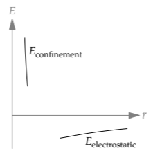
8.3.2.2 Hydrogen’s binding energy

Our next example, before we turn to the giant scales of stars, is our old friend the hydrogen atom. In Section 5.5.1, we predicted its size, the Bohr radius a₀, using dimensional analysis. The prediction was correct, but, as with the dimensional analysis of the atmosphere height, dimensional analysis didn’t give us a physical model. Easy-cases reasoning will help us make our tacit physical knowledge about hydrogen explicit and thereby build a physical model.

As we found in Section 6.5.2 using lumping, two physical effects compete:

1. Electrostatics. The electrostatic attraction between the proton and electron shrinks the atom.
2. Quantum mechanics. Via the uncertainty principle, quantum mechanics gives an electron confined to a small region a high momentum uncertainty and, therefore, a high kinetic energy. With this confinement energy, analogous to the thermal energy of an air molecule, the electron can resist the inward pull of electrostatics. Therefore, quantum mechanics expands the atom.

A dimensionless ratio that measures the relative size of the two effects is the energy ratio

\[\beta \equiv \frac{\vert \textrm{electrostatic potential energy} \vert}{\textrm{confinement energy}},\]

where the absolute-value bars say that, although the electrostatic potential energy is negative, we care only about its magnitude.

In a hydrogen atom of radius r, the electrostatic energy is \(e^{2}/4 \pi \epsilon_{0}r\). The confinement energy—which we estimated in Section 6.5.2 by using lumping—is comparable to \(\hbar^{2}/m_{e}r^{2}\). Therefore,

\[\beta \sim \frac{e^{2} 4 \pi \epsilon_{0} r}{\hbar ^{2}/m_{e}r^{2}}.\]

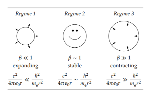
In the first regime, \(beta\) ≪ 1, quantum mechanics is much stronger than electrostatics, and the huge kinetic energy from quantum mechanics (the confinement energy) expands the atom. In the third regime, \(\beta\) ≫ 1, electrostatics, now much stronger than quantum mechanics, contracts the atom.

The radius of hydrogen, like the height of the atmosphere, is determined by the requirement that two physical effects compete and reach a draw. This truce happens in the middle regime. There, \(e^{2}/4 \pi \epsilon_{0} r \sim \hbar^{2}/m_{e}r^{2}\), so

\[r \sim \frac{\hbar^{2}}{m_{e}(e^{2}/4 \pi \epsilon_{0})},\]

which is the Bohr radius a₀ that we found using dimensional analysis (Section 5.5.1) and lumping (Section 6.5.2).

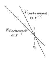
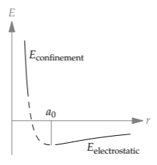
An alternative approach, which also uses easy cases but gives different insights, is to base the dimensionless ratio on the size r directly. Making r dimensionless requires another size. Fortunately, we have one, because the two energies, electrostatic and confinement, have different scaling exponents. The electrostatic energy is proportional to r⁻¹. The confinement energy is proportional to r⁻².

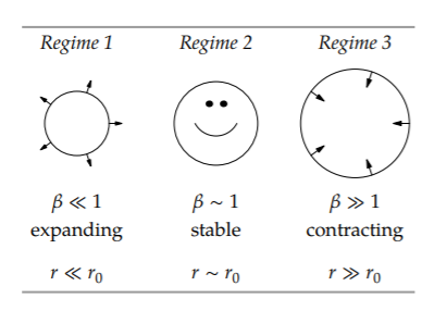
On log–log axes, they are straight lines but with different slopes: −2 for the confinement line and −1 for the electrostatic-energy line. Therefore, they intersect. The size at which they intersect is a special size. Let’s call it r₀. Then our dimensionless ratio is \(\beta \equiv r/r_{0}\), and the three regimes are shown in the table.

electrostatic and confinement energies, which is how we found the Bohr radius a₀ in Section 6.5.2. Thus, the radius of hydrogen is the Bohr radius and results from competition between electrostatics and quantum mechanics.

Our next project is to use the easy-cases regimes of size to understand thermal expansion—why substances expand upon heating. The first step is to sketch the total energy E, which is the sum of confinement and electrostatic energies

This sketch is easiest in the bookend regimes. In the first regime, where r ≪ r₀, the atom is too small, and quantum mechanics is stronger: Its kinetic-energy contribution is the dominant term in the energy, because its 1/r² scaling overwhelms the 1/r scaling of the potential energy. In the third regime, where r ≫ r₀, the atom is too large, and electrostatics is the dominant term in the energy: Its 1/r scaling goes to zero more slowly than the 1/r² scaling of the kinetic energy. Therefore, in the extremes (the bookends), the total energy has two different scalings:

\[ E \propto \left \{ \begin{array}{ll} 1/r^{2} (\textrm{regime 1}: r << r_{0}) \\ -1/r (\textrm{regime 3}: r >> r_{0}) \end{array} \right. \]

To complete the sketch, we interpolate between the bookend regimes.

The slopes in the two regimes have opposite signs, so there is no smooth way to connect the two extreme segments without introducing a point where the slope is zero. This point, where the energy is a minimum, is nature’s choice for the ground state of hydrogen.

With this sketch, we can explain thermal expansion. Thermal expansion first appeared in Problem 5.38, where you used dimensional analysis to estimate a typical thermal-expansion coefficient. However, the problem glided over the fundamental question: the coefficient’s sign. Knowing nothing about thermal expansion, we might guess that positive and negative coefficients are equally likely. Equivalently, substances are equally likely to expand as to contract when heated: Some substances might expand, and others might contract. However, this symmetry reasoning fails empirically: Almost all substances expand rather than contract when heated. The symmetry between positive and negative thermal-expansion coefficients, or between expansion and contraction, must get broken somewhere.

The curve of energy versus size for hydrogen shows where the symmetry gets broken. In its generic shape, the curve applies to all bonds, whether intra-atomic (such as the electron–proton bond in hydrogen), interatomic (such as hydrogen–oxygen bonds in a water molecule), or even intermolecular (such as the hydrogen bonds between water molecules). Bonds result from a competition between (1) attraction, which is important at long distances and which looks like the electrostatic piece of the generic curve, and (2) repulsion, which is important at short distances and which looks like the confinement piece of the generic curve. (Even the gravitational bond between the Sun and a planet, represented by the curve that you drew in Problem 5.55c, has the same shape.)

Therefore, the curve of bond energy versus separation cannot be symmetric. At the r ≪ r₀ end, which is the first regime, r has a minimum possible value, namely zero. However, at the r ≫ r₀ end, which is the third regime, r is unbounded. Thus, the two bookend regimes are not symmetric, and the bond-energy curve skews toward larger r.

To see how this asymmetry leads to thermal expansion, look at how thermal energy affects the average bond length. First, think of the bond as a spring (a model that we will discuss further in Section 9.1). As the bond vibrates around its equilibrium length r₀, thermal energy, which is a kinetic energy, converts into and out of potential energy in the bond. The minimum bond length r_min and the maximum bond length r_max are determined by where the vibration speed is zero—where the bond has slurped up all the kinetic energy (the thermal energy) and turned it into potential energy.

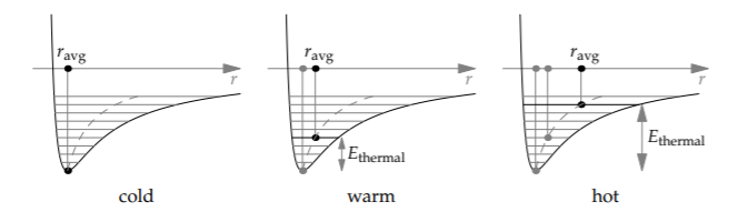
Graphically, we draw a horizontal line at a height E_thermal above the minimum energy. This line intersects the potential-energy curve twice, at r = r_min and at r = r_max. Because the potential-energy curve skews to the right, toward r ≫ r₀, the average bond length r_avg = (r_min + r_max)/2 is larger than r₀. As E_thermal grows, the skew affects the average more, and the difference between r_avg and r₀ grows: Adding thermal energy increases the bond length. Therefore, substances expand when heated.

8.3.2.3 Core temperature of the Sun

As our final example, we’ll estimate the temperature of the core of the Sun. The Sun, like the atmosphere, is a result of competition between thermal motion and gravity: Thermal motion expands the Sun; gravity compresses the Sun. A dimensionless measure of the two effects’ relative strength is

\[\beta \equiv \frac{\textrm{thermal energy}}{\vert \textrm{gravitational potential energy} \vert}.\]

The numerator, the thermal energy for one particle, is just k_BT. For the denominator, we need to know the mass of a particle. The Sun itself is made of hydrogen, but in the core of the Sun, the thermal energy is more than enough to strip an electron from the proton (as you verify in Problem 8.19). Each proton gets gravitational potential energy from the rest of the Sun, which has mass M_Sun. The rest of the Sun, if lumped into a massive particle, would be at a distance comparable to R_Sun, where R_Sun is the Sun’s radius. Therefore, the typical gravitational potential energy (per particle) is

\[E_{gravitational} \sim \frac{GM_{Sun}m_{p}}{R_{Sun}},\]

where the ∼ contains the minus sign in the potential energy. The ratio of energies is therefore

\[\beta \sim \frac{k_{B}T}{GM_{Sun}m_{p}/R_{Sun}},\]

and it produces the following three regimes.

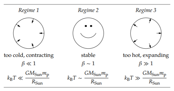
In the first regime, the Sun is too cold for its size, so gravity wins the competition and compresses the sun. This contraction shows the difference between the thermal–gravitational competition in the Sun and in the Earth’s atmosphere (Section 8.3.2.1). The temperature of the atmosphere is determined by the blackbody temperature of the Earth, roughly 300 K (Problem 5.43). In our analysis of the height of the atmosphere, we therefore held the temperature fixed and let only the height vary until it produced the gravitational energy to match the fixed thermal energy. In the Sun, however, the temperature is determined by the speed of the fusion reactions, which depends on the temperature and the density: Higher density means more frequent collisions that might result in fusion, and higher temperature (faster thermal motion) means that each collision has a higher chance of resulting in fusion. Thus, as the Sun contracts, the density increases, as does the temperature and the reaction rate. The contraction stops when the temperature is high enough for thermal motion to balance gravity.

(There is a caveat. If a star contracts very quickly, its core can heat up faster than the negative-feedback process can oppose the change. Then the core ignites like a giant hydrogen bomb and the star becomes a supernova.)

In the third regime, the Sun is too hot for its size, so thermal motion wins the competition and expands the Sun. As the Sun expands, the reaction rate, the temperature, and the thermal energy fall—until thermal motion again balances gravity. The result is the middle regime. In the middle regime, the Sun has just the right temperature—determined by the condition \(k_{B}T \sim GM_{Sun} m_{p}/R_{Sun},\), so

\[T \sim \frac{GM_{Sun}m_{p}}{k_{B}R_{Sun}}.\]

The proton mass m_p in the numerator and Boltzmann’s constant k_B in the denominator are easier to handle if we multiply each constant by Avogadro’s number N_A. The product N_Ak_B is the universal gas constant R. The product m_pN_A is the molar mass of protons, which is approximately the molar mass of hydrogen: 1 gram per mole. Then

\[T \sim \frac{\overbrace{6.7 \times 10^{-11} kg^{-1} m^{3} s^{-2}}^{G} \times \overbrace{2 \times 10^{30} kg}^{M_{Sun}} \times \overbrace{10^{-3} kg mol^{-1}}^{N_{A}m_{p}}}{\underbrace{8Jmol^{-1}K^{-1}}_{N_{A}k_{B}} \times \underbrace{0.7 \times 10^{9} m}_{R_{Sun}}}.\]

To evaluate T, start with the most important piece.

1. Units. The inverse moles in the numerator and denominator cancel. The numerator then contributes kg m³ s⁻², which is J m. The denominator contributes J K⁻¹ m. Therefore, the J m in the numerator and denominator cancel, and the inverse kelvins in the denominator become the kelvins in the Sun’s core temperature.
2. Powers of ten. The numerator contributes 16 powers of ten; the denominator contributes 9. The result is 7 powers of ten. Thus, the temperature will be comparable to 10⁷ K.
3. Numerical prefactor. The 6.7 in the numerator is mostly canceled out by the 8×0.7 in the denominator, leaving only the 2 in the numerator. Thus, the temperature is roughly 2×10⁷ K.

No one has measured the internal temperature directly, but the current best estimate for the core temperature is 1.5 × 10⁷ K. Our easy-cases model of competition between gravity and thermal motion is surprisingly accurate.

Exercise \(\PageIndex{12}\): Thermal versus electronic energy

Compare the thermal energy (per particle) in the core of the Sun to the binding energy of hydrogen. Were we justified in assuming that the electrons get stripped from the protons?