8.4: Two dimensionless quantities

In the examples of Section 8.3, one dimensionless quantity categorized the easy-cases regimes. Whether the quantity was small, comparable to 1, or large, the regimes could all be arranged on one axis. To extend that idea, we’ll use easy cases to categorize the world using two dimensionless quantities and therefore two axes. For practice, we’ll organize the world of waves onto a two-dimensional map (Section 8.4.1). Then we’ll organize the four fundamental branches of physics (Section 8.4.2).

8.4.1 The two-dimensional world of water waves

Water waves come in several varieties. Perhaps the most evident regime represents waves near a beach. These waves, the subject of Problem 5.15, have a wavelength much larger than the depth of the water. You can make them at home: Fill a bathtub or baking dish with water, disturb the water, and create waves sloshing back and forth. Their speed \(v\) is given by \(v^{2} = gh\), where h is the depth of the water.

Before these shallow-water waves reached the beach, they traveled on the open ocean, where their wavelength was much smaller than the depth. Their speed—technically, the phase velocity—is given by \(v^{2} g \cancel{\lambda}\) (Problem 5.11), where \(\cancel{\lambda}\) is the reduced wavelength \(\lambda/2 \pi\)

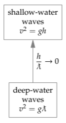
These two regimes—deep and shallow water—are distinguished by the dimensionless ratio \(h/\cancel{\lambda}\). (You can also use \(h/\lambda\), but the mathematical descriptions turn out to be simpler using \(h/\cancel{\lambda}\)) Therefore, the two regimes sit on a dimensionless axis that measures depth. Because the axis measures depth, let’s orient the axis vertically and place deep water at the bottom.

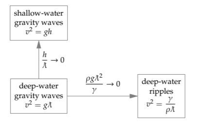
Another familiar kind of wave is produced by dropping a pebble in a pond. Small ripples zoom outward from the point of impact. These waves have a small wavelength, much smaller than the depth of the pond. Therefore, \(h/\cancel{\lambda}\) is large—as it is for deep-water waves.

However, these ripples are different from the deep-water waves on the open ocean. Ocean waves are driven by the water’s weight—that is, by gravity. In contrast, ripples are driven by the water’s surface tension—the same effect that allows small bugs to walk on water (see Problem 8.15). In order to distinguish ripples from deep-water gravity waves, our second axis should measure the relative importance of gravity and surface tension.

This axis is therefore labeled by the ratio of gravity to surface tension. This ratio is a dimensionless group, so we can find it using dimensional analysis. The ratio will depend on two characteristics of the water: its density {\rho} (to make the weight) and its surface tension \(\gamma\). It will depend on gravity g (to make the weight). And it will depend on the (reduced) wavelength \(\cancel{\lambda}\). These four quantities, built from three dimensions, form one independent dimensionless group. A useful choice is \(\rho g \cancel{\lambda}^{2}/\gamma\).

At long wavelengths (large \(\cancel{\lambda}\)), in dense fluids (large \(\rho\)), or in strong gravity (large g), this dimensionless ratio is large, indicating that gravity drives the waves. For short wavelengths (ripples) or, equivalently, high surface tension, this ratio is small, indicating that surface tension drives the waves. Here are the three regimes categorized using both groups.

The empty corner stares at us, asking to be filled. It incorporates both limits:

\[\frac{h}{\cancel{\lambda}} \rightarrow 0 \textrm{ (shallow water) and } \frac{\rho g \cancel{\lambda}^{2}}{\gamma} \rightarrow 0 \textrm{ (ripples).}\]

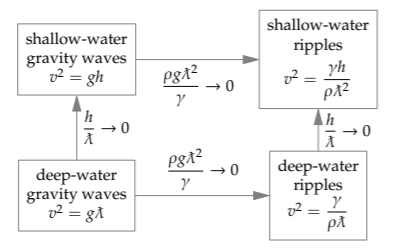
These waves are therefore ripples on shallow water. (They are hard to make, because ripples are tiny, smallerthan a few millimeters, yet the water depth must be even smaller.)

The four corners are the bookend regimes on two axes. If each axis had three regimes, two axes could have made three squared or nine regimes. The missing five middle regimes can be constructed by interpolating between the corners. The easy-cases map shows how: First fill in the four regions between the corners, and then fill in the center. That analysis, which involves addition and a tanh function, gives the following map.

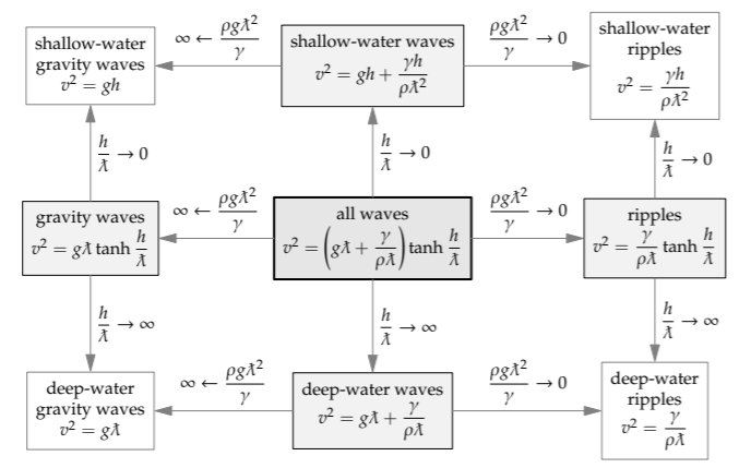
On this map, the middle regimes are not our usual middle regimes. Our usual middle regimes represented a particular regime (which was usually of the form \(\beta\) ∼ 1). However, on this map, the middle regimes represent the general solution \(\beta\) = anything. As an example, look at the bottom, deep-water row of three regimes. The bookend regimes, deep-water gravity waves and deep-water ripples, are easy cases of the middle, deep-water regime. For fun, check the other limiting cases, including that the central regime—which covers waves driven by any mixture of gravity and surface tension and traveling on any depth of water—turns into the other eight regimes in the appropriate limits.

8.4.2 The two-dimensional world of physics

Now we’ll use the same method to organize the four fundamental branches of physics: classical (Newtonian) mechanics, quantum mechanics, special relativity, and quantum electrodynamics.

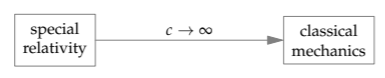
As a first step, which will determine the first axis, let’s compare classical mechanics and special relativity. Special relativity is Einstein’s theory of motion. It unifies classical mechanics and classical electrodynamics (the theory of radiation), giving a special role to the speed of light c. This role is popularized in the T-shirt showing Einstein in a policeman’s hat. He holds out his arm and palm to make a “Stop” signal and warns: “186 000 miles per second. It’s not just a good idea. It’s the law!” The speed of light is the universe’s speed limit, and special relativity obeys it. In contrast, classical mechanics knows no speed limit. Classical mechanics and special relativity therefore sit on an axis connected by the speed of light. In the limit c → ∞, special relativity turns into classical mechanics.

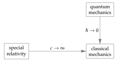
For the second axis, we compare one of the two remaining branches of physics—either quantum mechanics or quantum electrodynamics—with either classical mechanics or special relativity. Because quantum electrodynamics, if only from its name, looks frightening, let’s select quantum mechanics. We’ve seen its effect several times: Quantum mechanics contributes a new constant of nature \(\hbar\). This constant appears in the Heisenberg uncertainty principle \(\Delta p \Delta x \sim \hbar\), where \(\Delta p\) and \(\Delta x\) are a particle’s momentum and position uncertainties, respectively. The Heisenberg uncertainty principle restricts how small we can make these uncertainties, and therefore how accurately we can determine the position and momentum.

However, if \(\hbar\) were zero, then the uncertainty principle would not restrict anything. We could exactly determine the position and momentum of a particle simultaneously, as we expect in classical mechanics. Classical mechanics is the \(\hbar \rightarrow 0\) limit of quantum mechanics. Therefore, classical and quantum mechanics are connected on a second, \(\hbar\) axis. The map including quantum mechanics therefore has two dimensions.

In this two-dimensional map of physics, one corner sits empty. Furthermore, one branch of physics—quantum electrodynamics—hasn’t been considered. We need only a bit of courage to set quantum electrodynamics in the empty corner. Quantum mechanics must be the c → ∞ limit of quantum electrodynamics. And it is. Quantum electrodynamics is the result of marrying special relativity (c < ∞) and quantum mechanics (\(\hbar\) > 0). Thus, in the \(\hbar \rightarrow 0\) limit, quantum electrodynamics turns into special relativity.

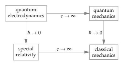
What happened to the bookend regimes?

The bookend regimes are here implicitly, because this example introduced a new feature: These axes are not labeled using dimensionless quantities! Only for a dimensionless quantity can we sensibly distinguish the three regimes ≪ 1, ∼ 1, and ≫ 1. Because c and ℏ have dimensions, the only valid comparisons are with zero or with infinity (which are zero and infinity in any system of units). Thus, there are only two regimes on each axis. The special-relativity–classical-mechanics axis compares c with infinity; the quantum-mechanics–classical-mechanics axis compares ℏ with zero.