9.3: Generating sound, light, and gravitational radiation

The sound generated by the vibrating wood blocks is an example of the most pervasive spring: radiation. It comes in three varieties. Electromagnetic radiation (or, more informally, light) is produced by an accelerating charge. Sound (acoustic radiation) can be produced simply by a changing but nonmoving charge (such as an expanding or contracting speaker membrane). Therefore, sound is simpler than light—which in turn is simpler than gravitational radiation. Do the easy cases first: We’ll first apply spring models to sound (Section 9.3.1). By adding the complexity of motion, we’ll extend the analysis to light (Section 9.3.2). Then we’ll be ready for the complexity of gravitational radiation (Section 9.3.3).

9.3.1 Acoustic radiation from a charge monopole

When we think of radiation, we think first of electromagnetic radiation, which we see (pun intended) everywhere. To analyze sound radiation while benefiting from what we know about electromagnetic radiation, we’ll find an analogy between electromagnetic and acoustic radiation—starting at the source of radiation, namely a single charge (a monopole).

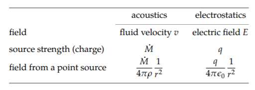
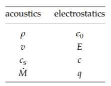
The search for the acoustic analog of charge is aided by scaling relations. An electric charge q produces a disturbance, the electric field E. Their connection is \(E \propto q\). Because the symbols E and q amplify the mental connection to electromagnetism, let’s write the relation between E and q in words. Words promote a broader, more abstract view not limited to electromagnetism:

\[\textrm{field} \propto \textrm{charge}.\]

Another transferable scaling comes from the energy density \(\varepsilon\) (energy per volume) in the field. For an electric field, \(\varepsilon \propto E^{2}\). In words,

\[\textrm{energy density} \propto \textrm{field}^{2}.\]

Sound waves move fluid, and motion means kinetic energy. Because the kinetic-energy density is proportional to the fluid velocity squared, the acoustic field could be the fluid velocity \(v\) itself. Then our first scaling relation, that field \(\propto\) charge, becomes

\[v \propto \textrm{charge}.\]

Thus, an acoustic charge moves fluid and with a speed proportional to the charge. In contrast to electromagnetism, acoustic charge cannot measure a fixed amount of stuff. For example, it cannot measure simply the volume of a speaker. A fixed volume would produce no motion and no acoustic field.

Instead, acoustic charge must measure a change in the source. As an example of such a change, imagine an expanding speaker. As it expands, it pushes fluid outward. The faster it expands, the faster the fluid moves. To identify the kind of change to measure, let’s work backward from the electric field E of a point electric charge to the velocity field \(v\) of a point acoustic charge. The electric field points outward with magnitude

\[E = \frac{q}{4 \pi \epsilon_{0} r^{2}}.\]

Futhermore, the electrostatic \(\epsilon_{0}\) appears in the energy density

\[\varepsilon = \frac{1}{2} \epsilon_{0} E^{2},\]

whose acoustic counterpart is the kinetic-energy density

\[\varepsilon = \frac{1}{2} \rho v^{2}.\]

Because \(E\) and \(v\) are analogous, the electrostatic \(\varepsilon_{0}\) corresponds, in acoustics, to the fluid density \(\rho\). Therefore, in the electric field, let’s replace \(\varepsilon_{0}\) by \(\rho\), \(E\) by \(v\), and \(q\) by acoustic charge to get

\[v = \frac{\textrm{acoustic charge}}{4 \pi \rho r^{2}},\]

or

\[\textrm{acoustic charge} = \frac{\rho v} \times 4 \pi r^{2}.\]

Here, r is the distance from the charge, and \(v\) is the fluid’s speed outward (just as the electric field points outward). Then each factor in the acoustic charge has a meaning, as does the product. The factor \(\rho v\) is the mass flux:

\[\underbrace{\textrm{flux}}_{\rho v} = \underbrace{\textrm{density of stuff}}_{\rho} \times \underbrace{\textrm{speed.}}_{v}\]

The factor \(4 \pi r^{2}\) is the surface area of a sphere of radius r. Thus, the acoustic charge \(\rho v \times 4 \pi r^{2}\) measures the rate at which mass flows out of this sphere.

The acoustic charge itself, at the center of this sphere, must displace mass at this rate. So the acoustic analog of charge is a mass source. The source could be an expanding speaker that directly forces fluid outward. Alternatively, it could be a hose supplying new fluid that forces the old fluid outward. For the rate, a convenient notation is \(\dot{M}\): The dot represents the time derivative, turning mass into a mass rate—which is the charge strength.

We have found an acoustic field \(v\) proportional to \(r^{-2}\). But, as we found in Section 5.4.3, the signature of radiation is that the field is proportional to \(r^{-1}\). So, we have constructed the acoustic analog of a static electric field and charge, but we have not yet constructed a radiating acoustic system

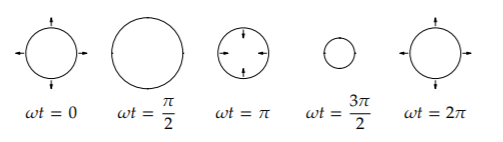
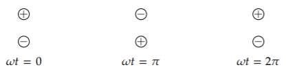
Producing radiation requires change—for example, due to a speaker. As a model of a speaker, a small pulsating sphere grows and shrinks in response to the music that it broadcasts. Maybe you put the sphere in a fancy box and slap a brand name on it, but growing and shrinking is still its fundamental operating principle and how it makes sound. A simple model of this change is spring motion—a sinusoidal oscillation in the charge:

\[\dot{M} = \dot{M}_{0} cos \omega t.\]

At t = 0, when \(cos \omega t = 1\), the speaker is expanding at its maximum rate, displacing mass at a rate \(\dot{M}_{0}\). At \(t = \pi/\omega\), the speaker is contracting at its maximum rate. Here is one cycle of its oscillation.

How much power does this changing acoustic charge radiate?

This analysis requires easy cases and lumping. Easy cases will help us find the velocity field; because the charge and field are changing, lumping will help us find the resulting energy flow. The easiest case is near the charge: News about the changes requires no time to arrive, so the fluid responds to a changing \(\dot{M}\) instantaneously. In this region, we know \(v\):

\[v = \frac{\dot{M}}{4 \pi \rho r^{2}}\]

Far from the charge, however, the fluid cannot know right away that \(\dot{M}\) has changed. But what does “far” mean? As we learned in Chapter 8, easy cases are defined by a dimensionless parameter, so the distance from the source is not enough information by itself to decide between near and far.

The decision needs a comparison length. This length is based on how the news is transmitted: It travels as a sound wave, so it has speed \(c_{s}\). Because the change happens at a rate \(\omega\) (the angular frequency of the charge oscillation), the characteristic timescale of the changes is \(\tau = 1/\omega\). In this time, the charge changes significantly, and the news has traveled a distance \(c_{s}\tau\) or \(\sim c_{s}/\omega\). This distance is the reduced wavelength \(\cancel{lambda}\) of the sound wave produced by the speaker (\(\cancel{\lambda} \equiv \lambda/2 \pi\)).

Therefore, "near the charge" (in the near field or zone) means \(r << \cancel{\lambda}\). "Far from the charge" (in the far field or the radiation field or zone) means \(r >> \cancel{\lambda}\). For examples, for middle C (\(f \approx 250\), and \(\lambda \approx 1.3\) meters), near and far are measured relative to 20 centimeters.

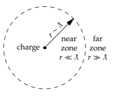
With \(\cancel{\lambda}\) as the comparison length, the dimensionless ratio determining whether r is small or large is \(r/\cancel{\lambda}\), which is \(r \omega/c_{s}\). At the boundary between the near and far zones, \(r \sim \cancel{\lambda}\).

To estimate the power carried by this signal—which is the power radiated by the source—start with the power per area, which is energy flux. At the zone boundary, \(r \sim \cancel{\lambda}\), so

\[\textrm{energy flux} = \underbrace{\textrm{energy density (at } r \sim \cancel{\lambda})}_{\rho v^{2}/2} \times \underbrace{\textrm{propagation speed.}}_{c_{s}}\]

To estimate the energy density at \(r \sim \cancel{\lambda}\), return to the lumping approximation—that the velocity field tracks the changes in \(\dot{M}\) throughout the near zone—and gather enough courage to extend the assumption. Assume that the instantaneous tracking happens all the way out to the zone boundary—that is, it applies not just when \(r << \cancel{\lambda}\) but even when \(r \sim \cancel{\lambda}\) (where the field abruptly changes its character and becomes a radiation field).

In this approximation, the velocity field at \(r \sim \cancel{\lambda}\) is

\[v \sim \frac{\dot{M}}{4 \pi \rho \cancel{\lambda}^{2}},\]

so the energy density \(\varepsilon \sim \rho v^{2}/2\) becomes

\[\varepsilon \sim \frac{1}{2} \rho(\frac{M}{4 \pi \rho \cancel{\lambda}^{2}})^{2}.\]

The radiating power P is the energy flux times the surface area of the sphere enclosing the near zone:

\[P \sim \underbrace{4 \pi \cancel{\lambda}^{2}}_{\textrm{surface area}} \times \underbrace{\frac{1}{2} \rho (\frac{\dot{M}}{4 \pi \rho \cancel{\lambda}^{2}})^{2}_{\textrm{energy density} \rho v^{2}/2} \times \underbrace{c_{s}.}_{\textrm{propagation speed}}\]

\[\cancel{\lambda} = c_{s}/\omega\), the power radiated by our acoustic monopole becomes

\[P_{\textrm{monopole}} = \frac{1}{8\pi} \frac{\dot{M}^{2} \omega^{2}}{\rho c_{s}}.\]

Despite the absurd number of lumping approximations, this result is exact! Let’s use it to estimate the acoustic power output of a tiny speaker.

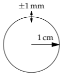
How much power is radiated by an \(R\) = 1 centimeter speaker whose radius varies by ±1 millimeter at \(f =1\) kilohertz (roughly two octaves above middle C)?

This calculation becomes slightly simpler if we replace \(\dot{M}\) by \(\rho \dot{V}\), where \(\dot{V}\) is the rate of volume change. (In acoustics, \(\dot{V}\) is often called the source strength Q—for example, in the classic work The Physics of Musical Instruments [15, p. 172]. However, for the sake of the analogy with electromagnetism, it is more consistent to make the source strength \(\dot{M}\) rather than \(\dot{V}\).) In terms of \(\dot{V}\),

\[P_{\textrm{monopole}} = \frac{1}{8 \pi} \frac{\rho \dot{V}^{2} \omega^{2}}{c_{s}}.\]

Here, \(\dot{V} = \dot{V}_{0} \textrm{cos} \omega t\), where \(\dot{V}_{0}\) is the amplitude of the oscillations in \(\dot{V}\). Therefore, the power P_monopole is also oscillating. By symmetry, the average value of \(\textrm{cos}^{2} \omega t\) is 1/2 (Problem 3.38), so the time-averaged power is one-half the maximum power:

\[P_{avg} = \frac{1}{16 \pi} \frac{\rho \dot{V}_{0}^{2} \omega^{2}}{c_{s}}.\]

To find the amplitude \(\dot{V}_{0}\), write \(\dot{V}\) in terms of the speaker dimensions:

\[\dot{V} = \underbrace{4 \pi R^{2}}_{\textrm{surface area}} \times v_{\textrm{surface}},\]

where v_surface is the outward speed of the speaker membrane. Because the surface is oscillating like a mass on a spring with amplitude A₀, its maximum velocity is \(A_{0}\omega\) and its time variation is

\[v_{surface} (t) = A_{0} \omega \textrm{cos} \omega t.\]

Then

\[\dot{V} = 4 \pi R^{2} A_{0} \omega \textrm{cos} \omega t.\]

The corresponding amplitude is everything except the cos \(\omega t\):

\[\dot{V}_{0} = 4 \pi R^{2} A_{0} \omega.\]

The radiated power is then

\[P_{avg} = \frac{1}{16 \pi} \frac{\rho \overbrace{(4 \pi R^{2} A_{0} \omega)^{2}}^{\dot{V}_{0}^{2}} \omega^{2}}{c_{s} = \frac{\pi \rho R^{4} A_{0}^{2} \omega ^{4}}{c_{s}}.\]

By multiplying P_avg by \(c_{s}^{3}/c_{s}^{3}\), the power can be written in terms of the dimensionless ratio \(R \omega/c_{s}\), which is also \(R/\cancel{\lambda}\):

\[P = \pi \rho c_{s}^{3}A_{0}^{2}(\frac{R \omega}{c_{s}})^{4} = \pi \rho c_{s}^{3} A_{0}^{2}(\frac{R}{\cancel{\lambda}})^{4}.\]

Physically, \(R/\cancel{\lambda}\) is the dimensionless speaker size (measured relative to \(\cancel{\lambda}\)). The scaling exponent of 4 tells us that the radiated power depends strongly on the dimensionless size of the speaker. As a result, big speakers (large R) are loud; and long wavelengths (low frequencies) require big speakers.

For this speaker, the radius is R is 1 centimeter, the surface-oscillation amplitude A₀ is 1 millimeter, and \(f\) is 1 kilohertz. So the wavelength of the sound is roughly 30 centimeters (\(\lambda = c_{s}/f\)), and \(\cancel{\lambda}\) is roughly 5 centimeters. Then the dimensionless speaker size \(R/\cancel{\lambda}\) is approximately 0.2, and

\[P_{avg} \approx \underbrace{3}_{\pi} \times \underbrace{1 \textrm{ kg m}^{-3}}_{\rho} \times \underbrace{(3 \times 10^{2} \textrm{ m s}^{-1})^{3}}_{c_{s}^{3}} \times \underbrace{(10^{-3})^{2}}_{A_{0}^{2}} \times \underbrace{0.2^{4}}_{(R/\cancel{\lambda})^{4}}.\]

To evaluate this power mentally, divide and conquer as usual:

1. Units. They are watts:

\[\textrm{kg m}^{-3} \times m^{3}s^{-3} \times m^{2} = \textrm{kg m}^{2} s^{-3} = W.\]

2. Powers of ten. They contribute 10⁻⁴:

\[\underbrace{{10^{6}}_{\textrm{from }c_{s}^{3}} \times \underbrace{10^{-6}}_{\textrm{from } A_{0}^{2}} \times \underbrace{10^{-4}}_{\textrm{from } (R/\cancel{\lambda})^{4}} = 10^{-4}.\]

So far, the power is 10⁻⁴ watts.

3. Remaining numerical factors. They are

\[\underbrace{3}_{\textrm{from } \pi} \times \underbrace{3^{3}}_{\textrm{from } c_{s}^{3}} \times \underbrace{2^{4}.}_{\textrm{from } (R/\cancel{\lambda})^{4}}\]

Because 2⁴=16 and 3 x 3³ is (3²)² or roughly 10², the remaining numerical factors contribute roughly 1600. Let's round it to 2000.

Then the power is roughly 2000 x 10^-4 or 0.2 watts.

Does that power represent a loud or a soft sound?

It depends on how close you stand to the speaker. If you are 1 meter away, the 0.2 watts are spread over a sphere of area \(4 \pi\) × (1 meter)², or roughly 10 square meters. Then the power flux is roughly 0.02 watts per square meter. In decibels, which is the more familiar measure of loudness (introduced in Problem 3.10), this power flux corresponds to just over 100 decibels, which is very loud, almost enough to cause pain.

What radius fluctuations would produce a barely audible, 0-decibel flux?

Shrinking the flux to 0 decibels, which is a drop of 100 decibels, is a drop of a factor of 10¹⁰ in energy flux and power. Because the energy flux is proportional to \(A_{0}^{2}\), A₀ must fall by a factor of 10⁵: from 10⁻³ meters to 10⁻⁸ meters. Thus, 10-nanometer fluctuations in a small speaker’s radius are (barely) enough to produce an audible sound. The human ear has an amazing dynamic range and sensitivity.

9.3.2 Electromagnetic radiation from a dipole

In the spirit of laziness, let’s transfer, by analogy, the radiated power from acoustic to electromagnetic radiation. In Section 9.3.1, we developed the analogy between acoustics and electrostatics. Using it, the acoustic radiated power,

\[P_{monopole} = \frac{1}{8 \pi} \frac{\dot{M}^{2} \omega^{2}}{\rho c_{s}},\]

implies an electromagnetic radiated power of \(q^{2} \omega^{2}/8 \pi \epsilon_{0}c.\)

Alas, this conjecture has three problems. First, if it represents the power radiated by an oscillating charge—moving, say, on a spring oscillating with frequency \(\omega\)—then its acceleration is \(\propto \omega^{2}\), so the radiated power is proportional to the acceleration. However, we learned from dimensional analysis (Section 5.4.3) that the power had to be proportional to the acceleration squared. Second, the power should depend on the amplitude of the motion, which is a length, yet the proposed power contains no such length.

These two problems are symptoms of the third problem, that transferring the acoustic analysis to electromagnetism has made an illegal situation. A single changing electromagnetic charge q(t) violates charge conservation: If q(t) is increasing, from where would the new charge come?

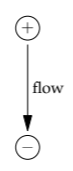
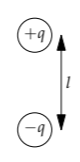
This question suggests the valid physical model, that the new charge comes from a nearby charge. As a model of this flow, imagine a pair of opposite, nearby charges. As the positive charge flows to the negative charge, the two charges swap places; and vice versa. This model is an oscillating dipole. Here is a full cycle of its oscillation.

If the charges are ±q and their separation is l, then ql is called their dipole moment d. Here, the time-varying dipole moment is \(d(t) = d_{0} \textrm{cos} \omega t\), where d₀ is the amplitude of the oscillations in the dipole moment. To estimate the power radiated, we’ll reuse the structure from acoustics,

\[P \sim \underbrace{4 \pi r^{2}}_{\textrm{surface area}} \times \underbrace{\frac{1}{2} \epsilon_{0}E^{2}}_{\textrm{energy density}} \times \underbrace{c,}_{\textrm{propagation speed}}\]

and evaluate it at the near-field–far-field boundary (\(r \sim \cancel{\lambda}\)). The only change from acoustics is that the electric field E is not the field from a single point charge (a monopole source) but rather from two opposite charges (a dipole source). Let’s evaluate their field at the position of a test charge at \(r \sim \cancel{\lambda}\).

The two charges (the monopoles) contribute slightly different electric fields E₊ and E_-. Because these fields are vectors, adding them correctly requires tracking their individual components. Let’s therefore make the lumping approximation that we can add the vectors using only their magnitudes:

\[E_{\textrm{dipole}} \approx E_{+} - E_{-}.\]

This approximation would be exact if the vectors lay along the same line—which they would if the dipole were an ideal dipole, with zero separation (l = 0). By making this approximation even for this nonideal dipole, we will obtain an important and transferable insight about the field of a dipole.

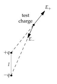
Because the distances from the test charge to the monopoles are almost identical, the two fields E₊ and E₋ have almost the same magnitude. Therefore, the difference E₊ − E₋ is almost zero. (The key word is almost. If the difference were exactly zero, there would be no light and no radiation.) Let’s approximate the difference using a further lumping approximation

The dipole field is the difference \(\Delta E = E(r_{+}) - E(r_{-})\), where E(r) is the monopole field. The difference is approximately

\[\underbrace{\Delta E}_{\textrm{rise}} \approx \underbrace{E'(r)}_{\textrm{slope}} \times \underbrace{\Delta r}_{\textrm{run}},\]

where \(\Delta r = r_{-} -r_{+}\). (This formula ignores a minus sign, but we are interested only in the magnitude of the field, so the sign doesn’t matter.) In Leibniz’s notation, the slope E′(r) is also dE/dr. Using the lumping approximation of Section 6.3.4 (which I remember as d ~ d), the d_s cancel and dE/dr, and therefore E′(r), is roughly E/r.

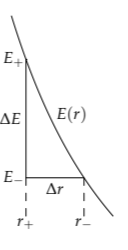
The trickiest factor is \(\Delta r\), which is \(r_{-} -r_{+}\). It depends on the charge separation l and on the position of the test charge relative to the dipole’s orientation. When the test charge is directly above the dipole (at the north pole), \(\Delta r\) is just the charge separation l. When the test charge is at the equator, \(\Delta r = 0\). With our lumping approximation, \(\Delta r\) is comparable to l.

Then the difference \(\Delta E\), which is the dipole field, becomes

\[E_{\textrm{dipole}} \sim E_{\textrm{monopole}} \times \frac{l}{r}.\]

The 1/r factor comes from differentiating the monopole field. The factor of l, the dipole size, turns the derivative of the field back into a field and makes the overall operation dimensionless: Making a dipole from two monopoles dimensionlessly differentiates the monopole field.

Because the energy density \(\varepsilon\) in the electric field is proportional to E², and the power radiated is proportional to the energy density, the power is

\[P_{dipole} \sim P_{monopole} (\frac{l}{r})^{2}.\]

In evaluating the radiated power, what \(r\) should we use?

The power radiated is determined by the energy density at the boundary between the near- and far-field regions: at \(r \sim c/\omega\). With that substitution,

\[P_{dipole} \sim \underbrace{\frac{1}{8\pi} \frac{q^{2}\omega^{2}}{\epsilon_{0}c}}_{P_{\textrm{monopole}}} \times (\frac{l}{c/\omega})^{2} = \frac{1}{\8 \pi}\frac{q^{2}l^{2}\omega^{4}}{\epsilon_{0}c^{3}}.\]

With a \(1/6 \pi\) instead of \(1/8 \pi\), this result is exact. Furthermore, if the source is a single accelerating charge, instead of a charge flow, then its acceleration is comparable to \(l \omega^{2}\), and \(P_{\textrm{dipole}} \sim q^{2}a^{2}/\epsilon_{0}c^{3}\), which is now consistent with what we derived in Section 5.4.3 using dimensional analysis.

In terms of the dipole moment \(d = ql\),

\[P_{\textrm{dipole}} = \frac{1}{6\pi} \frac{\omega^{4}d^{2}}{\epsilon_{0}c^{3}}.\]

Dipole radiation is the strongest kind of electromagnetic radiation. In Section 9.4, we’ll use the dipole power to explain why the sky is blue and a sunset red.

Exercise \(\PageIndex{1}\): Lifetime of hydrogen if it could radiate

Assuming that the ground state of hydrogen could radiate as an oscillating dipole (because of the orbiting electron), estimate the time \(\tau\) required for it to radiate its binding energy E₀. The ground state of hydrogen is protected by quantum mechanics—there is no lower-energy state to go to—but many of hydrogen’s higher-energy states have a lifetime comparable to \(\tau\).

9.3.3 Gravitational radiation from a quadrupole

Having started with acoustics and practiced with electromagnetics, we can extend our analysis of radiation to gravitational waves—without solving the equations of general relativity. In acoustics, radiation could be produced by a monopole (a point charge). In electromagnetics, radiation could be produced by a dipole but not by a monopole. Building a dipole requires charges of two signs. Because the gravitational equivalent of charge is mass, which comes in one sign, there is no way to make a gravitational dipole.

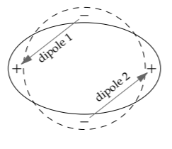
Therefore, gravitational radiation requires a quadrupole. A quadrupole is to a dipole what a dipole is to a monopole. It is two nearby dipoles with opposite strengths—so that their fields almost cancel.

An example is an oblate sphere. Relative to a sphere, it is fat at the equator (represented by the + signs) and thin at the poles (represented by the − signs). One plus–minus pair forms one dipole. The other plus–minus pair forms the second dipole. They have the same magnitude but point in opposite directions. As the sphere shifts to prolateness (tall and thin), the signs of the charges flip, as do the directions of the dipoles.

Just as the dipole field is the dimensionless derivative of the monopole field (Section 9.3.2), the quadrupole field is the dimensionless derivative of the dipole field. Thus, if the pulsating object has size l, so that the two dipoles are separated by a distance comparable to l, then at the boundary between the near and far fields (at \(r \sim c/\omega\)), the fields are related by

\[E_{\textrm{quadrupole}} \sim E_{\textrm{dipole}} \times \frac{l}{c/\omega} = E_{\textrm{dipole}} \times \frac{\omega l}{c}.\]

The radiated powers are related by the square of the extra factor:

\[P_{\textrm{quadrupole}} \sim P_{\textrm{dipole}} \times (\frac{\omega l}{c})^{2}.\]

That dimensionless ratio in parenthesis has a physical interpretation. Its numerator \(\omega l\) is the characteristic speed of the objects making the field. Its denominator c is the wave speed. Their ratio is the Mach number M, so \(\omega l/c\) is the characteristic Mach number of the sources. In terms of M,

\[P_{\textrm{quadrupole}} \sim P_{\textrm{dipole}} \times \textbf{M}^{2}.\]

For the radiated power from an electromagnetic dipole, we found an analogous relation:

\[P_{\textrm{dipole}} \sim P_{\textrm{monopole}} \times \textbf{M}^{2}.\]

In general,

\[P_{2^{m}-\textrm{pole}} \sim P_{\textrm{monopole}} \times \textbf{M}^{2m},\]

where a 2⁰-pole is a monopole, a 2¹-pole is a dipole, and so on.

With the analogy between electrostatics and gravity (from Section 2.4.2), we can convert the power radiated by an electromagnetic dipole to the power radiated by a gravitational dipole, if it existed. Then we just adjust for the difference between a dipole and a quadrupole. From the analogy, the electrostatic field E is analogous to the gravitational field g, and electrostatic charge q is analogous to mass m. Finally, because \(g= GM/r^{2}\) is analogous to \(E = q/4 \pi \epsilon_{0} r^{2}\), the electrostatic combination \(1/4 \pi \epsilon_{0}\) is analogous to Newton's constant G.

For electromagnetic dipole radiation, the power radiated is

\[P_{\textrm{dipole}} = \frac{1}{6 \pi \epsilon_{0}} \frac{q^{2}l^{2}\omega^{4}}{c^{3}}.\]

Replacing \(1/4 \pi \epsilon_{0}\) with G and q with m, but leaving c alone because gravitational waves also travel at the speed of light (a limitation set by relativity), the power radiated by a gravitational dipole, if it existed, would be

\[P_{\textrm{dipole}} \sim \frac{Gm^{2}l^{2}\omega^{4}}{c^{3}}.\]

Changing from dipole to quadrupole radiation adds a factor of \(\omega l/c\) to the field and \((\omega l/c)^{2}\) to the power, so

\[P_{\textrm{quadrupole}} \sim \frac{Gm^{2}l^{4}\omega^{6}}{c^{5}}.\]

Let’s use this formula to estimate the gravitational power radiated by the Earth–Sun system. We’ll divide the system into two sources. One source is the Earth as it rotates around the system’s center of mass (CM). The other source is the Sun as it rotates around the system’s center of mass.

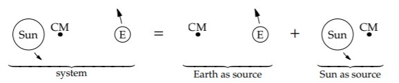
Which source generates more gravitational radiation?

The two sources share the constants of nature G and c. Because they orbit around the center of mass like a spinning dumbbell, they also share the angular velocity \(\omega\). Therefore, the power simplifies to a proportionality without G, c, or \(\omega\):

\[P_{\textrm{quadrupole}} \propto m^{2}l^{4},\]

where m is the mass of the object (either the Earth or Sun) and l is its distance from the center of mass. Furthermore, ml is shared, because the center of mass is defined as the point that makes ml the same for both objects.

\[m_{\textrm{Earth}} \times l_{\textrm{Earth-CM distance}} = M_{\textrm{Sun}} \times l_{\textrm{Sun-CM distance}}.\]

By factoring out two powers of ml and discarding them, the proportionality further simplifies from \(P_{\textrm{quadrupole} \propto m^{2}l^{4}\) to \(P_{\textrm{quadrupole}} \propto l^{2}\). The Earth, with the longer lever arm l, generates most of the gravitational wave energy. Equivalently, we can factor out four powers of ml and get \(P_{\textrm{quadrupole}} \propto m^{-2}\); the Earth, with the smaller mass, still wins. So

\[P_{\textrm{quadrupole}} \sim \frac{Gm^{2}_{\textrm{Earth}} l^{4} \omega^{6}}{c^{5}}.\]

As the last simplification before evaluating the power, let’s eliminate the angular frequency \(\omega\). For motion in a circle of radius \(l\), the centripetal acceleration is \(v^{2}/l\) (as we found in Section 5.1.1). In terms of the angular velocity, this acceleration is \(\omega^{2}/l\). It is produced by the gravitational force

\[F \approx \frac{GM_{\textrm{Sun}}m_{\textrm{Earth}}}{l^{2}}

(approximately, because lis slightly smaller than the Earth-Sun distance). The resulting cenripetal acceleration is \(F/m_{\textrm{Earth}}\) or \(GM_{\textrm{Sun}}/l^{2}\) so

\[\omega^{2} l = \frac{GM_{\textrm{Sun}}}{l^{2}}.\]

(approximately, because l is slightly smaller than the Earth-Sun distance). The resulting centripetal acceleration is \(F/m_{\textrm{Earth}}\) or \(GM_{\textrm{Sun}}/l^{2}\), so

\[\omega^{2}l = \frac{GM_{\textrm{Sun}}}{l^{2}}.\]

Using this relation to replace \((\omega^{2}l)^{3}\) in \(P_{\textrm{quadrupole}}\) with \((GM_{\textrm{Sun}}/l^{2})^{3}\) gives

\[P_{\textrm{quadrupole}} \sim \frac{G^{4}m^{2}_{\textrm{Earth}}M^{3}_{\textrm{Sun}}}{l^{5}c^{5}}.\]

The power based on a long and difficult general-relativity calculation is almost the same:

\[P_{\textrm{quadrupole}} \approx \frac{32}{5} \frac{G^{4}}{l^{5}c^{5}}(m_{\textrm{Earth}}M_{\textrm{Sun}})^{2}(m_{\textrm{Earth}} + M_{\textrm{Sun}}).\]

With the approximation that \(m_{\textrm{Earth}} + M_{\textrm{Sun}} \approx M_{\textrm{Sun}}\), the only difference between our estimate and the exact power is the dimensionless prefactor of 32/5. Including that factor and approximating \(m_{\textrm{Earth}} + M_{\textrm{Sun}}\) by \(M_{\textrm{Sun}}\),

\[P_{\textrm{quadrupole}} \approx \frac{32}{5} \frac{G^{4}m^{2}_{\textrm{Earth}}M^{3}_{\textrm{Sun}}}{l^{5}c^{5}}.\]

To avoid exponent whiplash and promote formula hygiene, let’s rewrite the power using a dimensionless ratio, by pairing another velocity with the c in the denominator. It would also be helpful to get rid of G, which seems like a random, meaningless value. To fulfill both wishes, we again equate the two ways of finding the Earth’s centripetal acceleration, as the acceleration produced by the Sun’s gravity and as the circular acceleration \(v^{2}/l\):

\[\frac{GM_{\textrm{Sun}}}{l^{2}} = \frac{v^{2}}{l}.\]

Therefore, \(GM_{\textrm{Sun}}/l = v^{2}\) and

\[\frac{G^{4}M^{4}_{\textrm{Sun}}}{l^{4}}= v^{8}.\]

That substitution gives

\[P_{\textrm{quadrupole}} \approx \frac{32}{5} \frac{m^{2}_{\textrm{Earth}}}{M_{\textrm{Sun}}} \frac{v^{8}}{lc^{5}}.\]

The ratio \(v^{5}/c^{5}\) is M⁵, where M is the Mach number of the Earth (its orbital velocity compared to the speed of light). Of the three remaining powers of \(v\), one power combines with l in the denominator to give back the angular velocity \(\omega = v/l\). The remaining two powers of \(v\) combine with one power of m_Earth to give (except for a factor of 2) the orbital kinetic energy of the Earth. The remaining masses make the Earth–Sun mass ratio m_Earth/M_Sun. Therefore, in a more meaningful form, the power is

\[P_{\textrm{quadrupole}} \approx \frac{32}{5} \frac{m_{\textrm{Earth}}}{M_{\textrm{Sun}}} \textbf{M}^{5} \times m_{\textrm{Earth}} v^{2} \omega.\]

In this processed form, the dimensions are more obviously correct than they were in the unprocessed form. The factors before the x sign are all dimensionless. The factor of m_Earthv² is an energy. And the factor of \(\omega\) converts energy into energy per time—which is power.

Now that we have reorganized the formula into meaningful chunks, we are ready to evaluate its factors.

1. The mass ratio is 3 x 10^-6:

\[\frac{m_{\textrm{Earth}}}{M_{\textrm{Sun}}} \approx \frac{6 \times 10^{24} \textrm{ kg}}{2 \times 10^{30} \textrm{ kg}} = 3 \times 10^{-6}.\]

2. The Mach number \(\textbf{M} \equiv v/c\) turns out to have a compact value. The Earth's orbital velocity \(v\) is 30 kilometers per second (Problem 6.5):

\[v = \frac{\textrm{circumference}}{\textrm{orbital period}} \approx \frac{2 \pi \times 1.5 \times 10^{11} m}{\pi \times 10^{7} s} = 3 \times 10^{4} \textrm{m s}^{-1},\]

which uses the estimate from Section 6.2.2 of the number of seconds in a year. The corresponding Mach number is 10^-4:

\[\textbf{M} \equiv \frac{v}{c} = \frac{3 \times 10^{4} \textrm{m s}^{-1}}{3 \times 10^{8} \textrm{m s}^{-1}} = 10^{-4}.\]

3. For the factor m_Earthv², we know m_Earth and have just evaluated v. The result is 6×10³³ joules:

\[\underbrace{6 \times 10^{24} kg}_{m_{\textrm{Earth}}} \times \underbrace{10^{9} m^{2} s^{-2}}_{v^{2}} = 6 \times 10^{33} J.\]

4. The final factor is the Earth’s orbital angular velocity \(\omega\). Because the orbital period is 1 year, \(\omega = 2 \pi/1\) year, or

\[\omega \approx \frac{2 \pi}{\pi \times 10^{7}s} = 2 \times 10^{-7} s^{-1}.\]

With these values,

\[P_{\textrm{quadrupole}} \approx \frac{32}{5} \times \underbrace{3 \times 10^{-6}}_{m_{\textrm{Earth}}/M_{\textrm{Sun}}} \times \underbrace{10^{-20}}_{\textbf{M}^{5}} \times \underbrace{6 \times 10^{33} J}_{m_{\textrm{Earth}}v^{2}} \times \underbrace{2 \times 10^{-7} s^{-1}.}_{\omega}\]

The resulting radiated power is about 200 watts. At that rate, the Earth’s orbit will not soon collapse due to gravitational radiation (Problem 9.8).

Quadrupole radiation depends strongly on the Mach number \(v_{\textrm{source}}/c\), and the Earth’s Mach number is tiny. However, when a star gets captured by a black hole, the orbital speed can be a large fraction of c. Then the Mach number is close to 1 and the radiated power can be enormous—perhaps large enough for us to detect on distant Earth.

Exercise \(\PageIndex{2}\): Energy loss through gravitational radiation

In terms of a gravitational system’s Mach number and mass ratio, how many orbital periods are required for the system to lose a significant fraction of its kinetic energy? Estimate this number for the Earth–Sun system.

Exercise \(\PageIndex{3}\): Gravitational radiation from the Earth-Moon system

Estimate the gravitational power radiated by the Earth–Moon system. Use the results of Problem 9.8 to estimate how many orbital periods are required for the system to lose a significant fraction of its kinetic energy.