9.4: Effect of radiation- Blue skies and red sunsets

We have developed almost all the pieces and tools to understand our final two phenomena: blue skies (Section 9.4.1) and red sunsets (Section 9.4.2). The only missing piece is the amplitude of a spring–mass system when it is driven by an oscillating force. We’ll build that piece where it is first needed, and then put all the pieces together.

9.4.1 Skies are blue

The light that we see from a clear sky is dipole radiation scattered from air molecules (on the Moon, with no atmosphere, there are no blue skies). Plenty of sunlight does not get affected by air molecules, but unless we look at the sun, which is almost always very hazardous, the direct sunlight does not reach our eye. (The exception is just at sunset, and in Section 9.4.2 we’ll use the exception to help explain why sunsets are red.

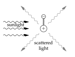
The analysis makes the most sense as a causal sequence from the sunlight to this scattered radiation. Sunlight is an oscillating electric field. The electric field exerts a force on the charged particles in an air molecule (say, in N₂). The charged particles, the electrons and protons, form spring–mass systems, and the electric force accelerates the masses. Accelerating charges radiate, which is the radiation that reaches our eye. By quantifying the steps in the sequence from sunlight to scattered radiation, we’ll see why the scattered radiation looks blue.

1. Electric field of the sunbeam. Sunlight contains many colors of light, each simple to describe as an electric field (divide and conquer!):

\[E(\omega) = E_{0} (\omega) \textrm{cos} \omega t,\]

where \(\omega\) is the angular frequency corresponding to that color. For example, for red light, \(\omega\) is 3 × 1015 radians per second. The amplitude \(E_{0}(\omega)\) depends on the intensity of the color in sunlight, so \(E(\omega)\) is a distribution over \(\omega\), and it and the amplitude \(E_{0}(\omega)\) have dimensions of field per frequency. However, as a simple lumping approximation, think of seven separate fields, one for each color in the color mnemonic Roy G. Biv: red, orange, yellow, green, blue, indigo, and violet.

For the color of the sky, what matters is the relative distribution of colors in the sunbeam and how that relative distribution is different in scattered light. Therefore, let’s do our calculations in terms of an unknown E₀ and, in the spirit of proportional reasoning, determine the dependence of E₀ on \(\omega\) in the scattered light.

2. Force on the charged particles. The electric field produces a force on the electrons and protons in an air molecule. Using e for the electron charge and ignoring signs,

\[F = eE = eE_{0} \textrm{cos} \omega t,\]

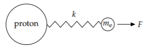
3. Amplitude of the motion of the charged particles. Because protons are much heavier than an electrons, the electrons move faster and farther than the protons and produce most of the scattered radiation. Therefore, let’s assume that the protons are fixed and analyze the motion of an electron.

The electron, which is connected to its proton by a spring, is driven by the oscillating force F. Fortunately, we do not need to solve for the motion, in general, because we can use easy cases based on the ratio between the driving frequency \(\omega\) and the system’s natural frequency \(\omega_{0}\) (which is \(\sqrt{k/m_{e}}\), where k is the bond’s spring constant). The three regimes are then (1) \(\omega << \omega_{0}\), (2) \(\omega = \omega_{0}\), and (3) \(\omega >> \omega_{0}\).

To decide which regime is relevant, let’s make a rough estimate of how the two frequencies compare. For air molecules, the natural frequency \(\omega_{0}\) corresponds to ultravioletradiation—the radiation required to break the strong triple bond in N₂. The driving frequency \(\omega\) corresponds to one of the colors in visible light (sunlight), so the electron’s motion is in the first, low-frequency regime \(\omega << \omega_{0}\). (For the analysis of the other regimes, try Problems 9.12 and 9.15.) The low-frequency regime is easiest to study in the \(\omega = 0\) extreme. It represents a constant force \(F = eE_{0}\) pulling on the electron and stretching the electron–proton bond. When there is change, make what does not change! The bond stretches until the spring force balances the stretching force \(eE_{0}\). The forces balance when the stretch is \(x = F/k\) or \(eE_{0}/k\).

Because \(\omega = 0\), the force has been constant since forever, so the bond stretched to its extended length back in the mists of time. When \(\omega\) is nonzero, but still much smaller than \(\omega_{0}\), the bond still behaves approximately as it did when \(\omega = 0\): It stretches so that the spring force balances the slowly oscillating force F. Therefore, the stretch, which is the displacement of the electron, is

\[x(t) \approx \frac{eE_{0}}{k} \textrm{cos} \omega t.\]

4. Acceleration of the electron. We can find the acceleration using dimensional analysis. In driven spring motion, the important length is the displacement x, and the important time is \(1/\omega\). Therefore, the acceleration, which has dimensions of LT⁻², must be comparable to \(x \omega^{2}\). Because we used the angular frequency (\(\omega\) rather than \(f\)), the dimensionless prefactor turns out to be 1. Then the electron’s acceleration is

\[a(t) = x(t) \omega^{2} \approx \frac{eE_{0}\omega^{2}}{k} \textrm{cos} \omega t.\]

Because the spring constant k is related to the electron mass m_e and to the natural frequency \(\omega_{0}\) by \(k=m_{e}\omega_{0}^{2}\),

\[a(t) \approx \frac{eE_{0}}{m_{e}}\frac{\omega^{2}}{\omega_{0}^{2}} \textrm{cos} \omega t.\]

5. Power radiated by the accelerating electron. We found in Sections 5.4.3 and 9.3.2 that the power radiated by an accelerating charge e is

\[P_{\textrm{dipole}} = \frac{e^{2}}{6 \pi \epsilon_{0}} \frac{a^{2}}{c^{3}}.\]

For the squared acceleration \(a^{2}\), we'll use the time average to find the average radiated power. Because the time average of \(\textrm{cos}^{2}\omega t\) is 1/2,

\[\langle a^{2} \rangle = \frac{1}{2} \frac{e^{2} E_{0}^{2}}{m_{e}^{2}} \frac{\omega^{4}}{\omega_{0}^{4}}.\]

Then

\[P_{\textrm{dipole}} = \frac{1}{12 \pi \epsilon_{0}} \frac{1}{c^{3}} \frac{e^{4}E_{0}^{2}}{m_{e}^{2}} (\frac{\omega}{\omega_{0}})^{4}.\]

This mouthful is useful in explaining the color of sunsets (Section 9.4.2), so it has been worthwhile carrying lots of baggage on the trip from sunlight to scattered light. But to explain the color of the daytime sky, we can simplify the power using proportional reasoning. Because \(\epsilon_{0}\), c, \(\omega_{0}\), m_e, and e are independent of the driving frequency \(\omega\) (which represents the color),

\[P_{\textrm{dipole}} \propto E_{0}^{2}\omega^{4}\]

The factor of \(E_{0}^{2}\) is proportional to the energy density in the incoming sunlight (at frequency \(\omega\)), which itself is proportional to the incoming power in the sunlight (also at the frequency \(\omega\)). Thus,

\[P_{\textrm{dipole}} \propto P_{\textrm{sunlight}} \omega^{4}.\]

Let’s review how the four powers of \(\omega\) got here. For low frequencies—and visible light is a low frequency compared to the natural electronic-vibration frequency of an air molecule—the amplitude of spring motion is independent of the driving frequency. The acceleration is then proportional to \(\omega^{2}\). And the radiated power is proportional to the square of the acceleration, so it is proportional to \(\omega^{4}\).

Therefore, the air molecule acts like a filter that takes in (some of the) incoming sunlight and produces scattered light, altering the distribution of colors—similar to how a circuit changes the amplitude of each incoming frequency. However, unlike the low-pass RC circuit of Section 2.4.4, which preserves low frequencies and attenuates high frequencies, the air molecule amplifies the high frequencies.

Here are the sunlight and the scattered spectra based on the \(\omega^{4}\) filter. Each spectrum shows, by the area of each band, the relative intensities of the various colors. (The unlabeled color band between red and yellow is orange.)

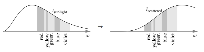
Sunlight looks white. In the scattered light, the high-frequency colors such as blue and violet are much more prominent than they are in sunlight. For example, because \(\omega_{\textrm{blue}}/\omega_{\textrm{red}} \approx 1.5\) and 1.5⁴ ≈ 5, the blue part of the sunlight is amplified by a factor of 5 compared to the red part. As a result, the scattered light—what comes to us from the sky—looks blue!

9.4.2 Sunsets are red

As sunlight passes through the atmosphere, ever more of its energy gets taken in by air molecules and then scattered (reradiated) in all directions. As we found in Section 9.4.1, this process happens more rapidly at higher (bluer) frequencies, due to the factor of \(\omega^{4}\) in the radiated power. Therefore, the sunbeam becomes redder as it travels through the atmosphere. If the beam travels far enough in the atmosphere, sunsets should look red. To estimate the necessary travel distance, we can adapt the analysis of Section 9.4.1. Then we will use geometry to estimate the actual travel distance

How far must sunlight travel in the atmosphere before the beam looks red?

To estimate this length, let’s estimate the rate at which energy gets scattered out of the beam. The beam carries an energy flux

\[F = \frac{1}{2} \epsilon_{0}E_{0}^{2}c,\]

which has the usual form of energy density times propagation speed. (The electric and magnetic fields each contribute one-half of this flux.) To measure the effect of one scattering electron on the beam, let’s compute one electron’s radiated power divided by the flux:

\[\frac{P_{\textrm{dipole}}}{F} = \underbrace{\frac{1}{12 \pi \epsilon_{0}} \frac{1}{c^{3}} \frac{e^{4}\cancel{E_{0}^{2}}}{m_{e}^{2}}(\frac{\omega}{\omega_{0}})^{4}}_{P_{\textrm{dipole}}} / \underbrace{\frac{1}{2} \epsilon_{0} \cancel{E_{0}^{2}}c.}_{F}\]

Noticing that the (unknown) field amplitude E₀ cancels out and doing the rest of the algebra, we get

\[\frac{P_{\textrm{dipole}}}{F} = \underbrace{\frac{8 \pi}{3} (\frac{e^{2}}{4 \pi \epsilon_{0}} \frac{1}{m_{e}c^{2}})^{2}}_{\textrm{area } \sigma} \times (\frac{\omega}{\omega_{0}})^{4}.\]

The left side, P_dipole/F, is power divided by power per area. Thus, P_dipole/F has dimensions of area. It represents the area of the beam whose energy flux gets removed and scattered in all directions. The area is therefore called the scattering cross section \(\sigma\) (a concept introduced in Section 6.4.5, when we estimated the mean free path of air molecules).

On the right side, the frequency ratio \(\omega/\omega_{0}\) is dimensionless, so the prefactor must also be an area. It is called the Thomson cross section \(\sigma_{T}\):

\[\sigma_{T} \equiv \frac{8 \pi}{3} (\frac{e^{2}}{4 \pi \epsilon_{0}}\frac{1}{m_{e}c^{2}})^{2} \approx 7 \times 10^{-29} m^{2}.\]

Because \(\sigma_{T}\) is an area, the factor inside the parentheses must be a length. Indeed, it is the classical electron radius r₀ of Problems 5.37 and 5.44(a). It is comparable to the proton radius of 10−15 meters:

\[r_{0} \equiv \frac{e^{2}}{4 \pi \epsilon_{0}} \frac{1}{m_{e}c^{2}} \equiv 2.8 \times 10^{-15} m.\]

It approximately answers the question: For the electron to acquire its mass from its electrostatic energy, how large should the electron be? This electron’s cross-sectional area is, roughly, the Thomson cross section. In terms of the Thomson cross section, our scattering cross section \(\sigma\) is

\[\sigma = \sigma_{T}(\frac{\omega}{\omega_{0}})^{4}.\]

Each scattering electron converts this much area of the beam into scattered radiation. As a rough estimate, each air molecule contributes one scattering electron (the inner electrons, which are tightly bound to the nucleus, have a large \(\omega_{0}\) and a tiny scattering cross section). As we found in Section 6.4.5, the mean free path \(\lambda_{mfp}\) and scattering cross section \(\sigma\) are related by

\[n \sigma \lambda_{mfp} \sim 1,\]

where n is the number density of scattering electrons. The mean free path is how far the beam travels before a significant fraction of its energy (at that frequency) is scattered in all directions and is no longer part of the beam.

With one scattering electron per air molecule, n is the number density of air molecules. This number density, like the mass density, varies with the height above sea level. To simplify the analysis, we will use a lumped atmosphere. It has a constant temperature, pressure, and density from sea level to the atmosphere’s scale height H, which we estimated in Section 5.4.1 using dimensional analysis (and you estimated using lumping in Problem 6.36). At H, the atmosphere ends, and the density abruptly goes to zero.

In this lumped atmosphere, 1 mole of air molecules at any height occupies approximately 22 liters. The resulting number density is approximately 3×10²⁵ molecules per cubic meter:

\[n = \frac{1 \textrm{ mol}}{22 l} \times \frac{6 \times 10^{23}}{1 \textrm{ mol}} \times \frac{10^{3} l}{1 m^{3}} \approx 3 \times 10^{25} m^{-3}.\]

Using this n and \(\sigma = \sigma_{T}(\omega/\omega_{0})^{4}\), the mean free path becomes

\[\lambda_{mfp} \sim \frac{1}{n \sigma} \approx \frac{1}{\underbrace{3 \times 10^{25} m^{-3}}_{n}} \times \frac{1}{\underbrace{7 \times 10^{-29} m^{2}}_{\sigma_{T}}} \times (\frac{\omega_{0}}{\omega})^{4} \approx \frac{1}{2} \textrm{ km} \times (\frac{\omega_{0}}{\omega})^{4}.\]

Unlike the scattering cross section \(\sigma\), which grows rapidly with \(\omega\), the mean free path falls rapidly with \(\omega\): High frequencies scatter out of the beam rapidly and travel shorter distances before getting significantly attenuated.

To estimate the frequency ratio \(\omega_{0}/\omega\), let’s estimate the equivalent energy ratio \(\hbar \omega_{0}/\hbar \omega\). The numerator \(\hbar \omega_{0}\) is the bond energy. Because air is mostly N₂, and the nitrogen–nitrogen triple bond is much stronger than a typical chemical bond (roughly 4 electron volts), the natural frequency \(\omega_{0}\) corresponds to an energy \(\hbar \omega_{0}\) of about 10 electron volts.

The denominator \(\hbar \omega\) depends on the color of the light. As a lumping approximation, let’s divide light into two colors: red and, to represent nonred light, blue–green light. A blue–green photon has an energy \(\hbar \omega\) of approximately 2.5 electron volts, so \(\hbar \omega_{0}/\hbar \omega \approx 4\) and \((\omega_{0}/\omega)^{4} \approx 200\). Because the mean free path is

\[\lambda_{mfp} \approx \frac{1}{2} km \times (\frac{\omega_{0}}{\omega})^{4},\]

for blue–green light \(\lambda_{mfp} \sim 100\) kilometers. After a distance comparable to 100 kilometers, a significant fraction of the nonred light has been removed (and scattered in all directions).

At midday, when the Sun is overhead, the travel distance is the thickness of the atmosphere H, roughly 8 kilometers. This distance is much shorter than the mean free path, so very little light (of any color) is scattered out of the sunbeam, and the Sun looks white as it would from space. (Fortunately, our theory doesn’t predict that the midday Sun looks red—but do not test this analysis by looking directly at the Sun!) As the Sun descends in the sky, sunlight travels ever farther in the atmosphere.

At sunset, how far does sunlight travel in the atmosphere?

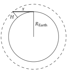
This length is the horizon distance: Standing as high as x the atmosphere (H ≈ 8 kilometers), the horizon distance x is the distance that sunlight travels through the atmosphere at sunset. It is the geometric mean of the atmosphere height H and of the Earth’s diameter 2R_Earth (Problem 2.9), and is approximately 300 kilometers:

\[x = \sqrt{H \times 2R_{\textrm{Earth}}} \approx \sqrt{8 km \times 2 \times 6000 km} \approx 300 km. \]

This distance is a few mean free paths. Each mean free path produces a significant reduction in intensity (more precisely, a factor-of-e reduction). Therefore, at sunset, most of the non-red light is gone.

However, for red light the story is different. Because a red-light photon has an energy of approximately 1.8 electron volts, in contrast to the 2.5 electron volts for a blue-green photon, its mean free path is a factor of (2.5/1.8)⁴ ≈ 4 longer than 100 kilometers for a blue–green photon. The trip of 300 kilometers in the atmosphere scatters out a decent fraction of red light, but much less than the corresponding fraction of blue–green light. The moral of the story is visual: Together the springs in the air molecules and the steep dependence of dipole radiation on frequency produce a beautiful red sunset.