10.3: Eigenvalues and Eigenvectors
- Page ID
- 22501
What are Eigenvectors and Eigenvalues?
Eigenvectors ( ) and Eigenvalues (\(λ\)) are mathematical tools used in a wide-range of applications. They are used to solve differential equations, harmonics problems, population models, etc. In Chemical Engineering they are mostly used to solve differential equations and to analyze the stability of a system.
- An Eigenvector is a vector that maintains its direction after undergoing a linear transformation.
- An Eigenvalue is the scalar value that the eigenvector was multiplied by during the linear transformation.
Eigenvectors and Eigenvalues are best explained using an example. Take a look at the picture below.
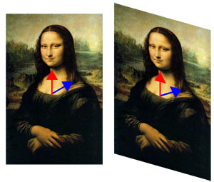
In the left picture, two vectors were drawn on the Mona Lisa. The picture then under went a linear transformation and is shown on the right. The red vector maintained its direction; therefore, it’s an eigenvector for that linear transformation. The blue vector did not maintain its director during the transformation; thus, it is not an eigenvector. The eigenvalue for the red vector in this example is 1 because the arrow was not lengthened or shortened during the transformation. If the red vector, on the right, were twice the size than the original vector then the eigenvalue would be 2. If the red vector were pointing directly down and remained the size in the picture, the eigenvalue would be -1.
Now that you have an idea of what an eigenvector and eigenvalue are we can start talking about the mathematics behind them.
Fundamental Equation
The following equation must hold true for Eigenvectors and Eigenvalues given a square matrix \(\mathrm{A}\):
\[\mathrm{A} \cdot \mathrm{v}=\lambda \cdot \mathrm{v} \label{eq1} \]
where:
- \(\mathrm{A}\) is a square matrix
- \(\mathrm{v}\) is the Eigenvector
- \(\lambda\) is the Eigenvalue
Let's go through a simple example so you understand the fundamental equation better.
Is \(\mathbf{v}\) an eigenvector with the corresponding \(λ = 0\) for the matrix \(\mathbf{A}\)?
\[\mathbf{v}=\left[\begin{array}{c} 1 \\ -2 \end{array}\right] \nonumber \nonumber \]
\[\mathbf{A}=\left[\begin{array}{cc} 6 & 3 \\ -2 & -1 \end{array}\right] \nonumber \nonumber \]
Solution
\[\begin{align*} A \cdot \mathbf{v} &= \lambda \cdot \mathbf{v} \\[4pt] \left[\begin{array}{cc} 6 & 3 \\ -2 & -1 \end{array}\right] \cdot\left[\begin{array}{c} 1 \\ -2 \end{array}\right] &=0\left[\begin{array}{c} 1 \\ -2 \end{array}\right] \\[4pt] \left[\begin{array}{l} 0 \\ 0 \end{array}\right] &=\left[\begin{array}{l} 0 \\ 0 \end{array}\right] \end{align*}\nonumber \]
Therefore, it is true that \(\mathbf{v}\) and \(λ = 0\) are an eigenvector and eigenvalue respectively, for \(\mathbf{A}\). (See section on Matrix operations, i.e. matrix multiplication)
Calculating Eigenvalues and Eigenvectors
Calculation of the eigenvalues and the corresponding eigenvectors is completed using several principles of linear algebra. This can be done by hand, or for more complex situations a multitude of software packages (i.e. Mathematica) can be used. The following discussion will work for any nxn matrix; however for the sake of simplicity, smaller and more manageable matrices are used. Note also that throughout this article, boldface type is used to distinguish matrices from other variables.
Linear Algebra Review
For those who are unfamiliar with linear algebra, this section is designed to give the necessary knowledge used to compute the eigenvalues and eigenvectors. For a more extensive discussion on linear algebra, please consult the references.
Basic Matrix Operations
An m x n matrix A is a rectangular array of \(mn\) numbers (or elements) arranged in horizontal rows (m) and vertical columns (n):
\[\boldsymbol{A}=\left[\begin{array}{lll}
a_{11} & a_{1 j} & a_{1 n} \\
a_{i 1} & a_{i j} & a_{i n} \\
a_{m 1} & a_{m j} & a_{m n}
\end{array}\right]\nonumber \]
To represent a matrix with the element aij in the ith row and jth column, we use the abbreviation A = [aij]. Two m x n matrices A = [aij] and B = [bij] are said to be equal if corresponding elements are equal.
Addition and subtraction
We can add A and B by adding corresponding elements:
\[A + B = [a_{ij}] + [b_{ij}] = [a_{ij} + b_{ij}\nonumber \]
This will give the element in row i and column j of C = A + B to have
\[c_{ij} = a_{ij} + b_{ij}.\nonumber \]
More detailed addition and subtraction of matrices can be found in the example below.
\[\left[\begin{array}{ccc}
1 & 2 & 6 \\
4 & 5 & 10 \\
5 & 3 & 11
\end{array}\right]+\left[\begin{array}{ccc}
8 & 3 & 5 \\
5 & 4 & 4 \\
3 & 0 & 6
\end{array}\right]=\left[\begin{array}{ccc}
1+8 & 2+3 & 6+5 \\
4+5 & 5+4 & 10+4 \\
5+3 & 3+0 & 11+6
\end{array}\right]=\left[\begin{array}{ccc}
9 & 5 & 11 \\
9 & 9 & 14 \\
8 & 3 & 17
\end{array}\right]\nonumber \]
Multiplication
Multiplication of matrices are NOT done in the same manner as addition and subtraction. Let's look at the following matrix multiplication:
\[A \times B=C\nonumber \]
\(A\) is an \(m \times n\) matrix, \(B\) is an \(n \times p\) matrix, and \(C\) is an \(m \times p\) matrix. Therefore the resulting matrix, \(C\), has the same number of rows as the first matrix and the same number of columns as the second matrix. Also the number of columns in the first is the same as the number of rows in the second matrix.
The value of an element in C (row i, column j) is determined by the general formula:
\[c_{i, j}=\sum_{k=1}^{n} a_{i, k} b_{k, j}\nonumber \]
Thus,
\[\begin{align*} \left[\begin{array}{ccc}
1 & 2 & 6 \\
4 & 5 & 10 \\
5 & 3 & 11
\end{array}\right]\left[\begin{array}{cc}
3 & 0 \\
0 & 1 \\
5 & 1
\end{array}\right] &=\left[\begin{array}{cc}
1 \times 3+2 \times 0+6 \times 5 & 1 \times 0+2 \times 1+6 \times 1 \\
4 \times 3+5 \times 0+10 \times 5 & 4 \times 0+5 \times 1+10 \times 1 \\
5 \times 3+3 \times 0+11 \times 5 & 5 \times 0+3 \times 1+11 \times 1
\end{array}\right] \\[4pt] &=\left[\begin{array}{cc}
33 & 8 \\
62 & 15 \\
70 & 14
\end{array}\right]\end{align*} \nonumber \]
It can also be seen that multiplication of matrices is not commutative (A B ≠B A). Multiplication of a matrix by a scalar is done by multiplying each element by the scalar.
cA = Ac =[caij]
\[2\left[\begin{array}{ccc}
1 & 2 & 6 \\
4 & 5 & 10 \\
5 & 3 & 11
\end{array}\right]=\left[\begin{array}{ccc}
2 & 4 & 12 \\
8 & 10 & 20 \\
10 & 6 & 22
\end{array}\right]\nonumber \]
Identity Matrix
The identity matrix is a special matrix whose elements are all zeroes except along the primary diagonal, which are occupied by ones. The identity matrix can be any size as long as the number of rows equals the number of columns.
\[\mathbf{I}=\left[\begin{array}{llll}
1 & 0 & 0 & 0 \\
0 & 1 & 0 & 0 \\
0 & 0 & 1 & 0 \\
0 & 0 & 0 & 1
\end{array}\right]\nonumber \]
Determinant
The determinant is a property of any square matrix that describes the degree of coupling between equations. For a 2x2 matrix the determinant is:
\[\operatorname{det}(\mathbf{A})=\left|\begin{array}{ll}
a & b \\
c & d
\end{array}\right|=a d-b c\nonumber \]
Note that the vertical lines around the matrix elements denotes the determinant. For a 3x3 matrix the determinant is:
\[\operatorname{det}(\mathbf{A})=\left|\begin{array}{lll}
a & b & c \\
d & e & f \\
g & h & i
\end{array}\right|=a\left|\begin{array}{cc}
e & f \\
h & i
\end{array}\right|-b\left|\begin{array}{cc}
d & f \\
g & i
\end{array}\right|+c\left|\begin{array}{cc}
d & e \\
g & h
\end{array}\right|=a(e i-f h)-b(d i-f g)+c(d h-e g)\nonumber \]
Larger matrices are computed in the same way where the element of the top row is multiplied by the determinant of matrix remaining once that element’s row and column are removed. Terms where the top elements in odd columns are added and terms where the top elements in even rows are subtracted (assuming the top element is positive). For matrices larger than 3x3 however; it is probably quickest to use math software to do these calculations since they quickly become more complex with increasing size.
Solving for Eigenvalues and Eigenvectors
The eigenvalues (λ) and eigenvectors (v), are related to the square matrix A by the following equation. (Note: In order for the eigenvalues to be computed, the matrix must have the same number of rows as columns.)
\[(\mathbf{A}-\lambda \mathbf{I}) \cdot \mathbf{v}=0\nonumber \]
This equation is just a rearrangement of the Equation \ref{eq1}. To solve this equation, the eigenvalues are calculated first by setting det(A-λI) to zero and then solving for λ. The determinant is set to zero in order to ensure non-trivial solutions for v, by a fundamental theorem of linear algebra.
\[A=\left[\begin{array}{lll}
4 & 1 & 4 \\
1 & 7 & 1 \\
4 & 1 & 4
\end{array}\right]\nonumber \]
\[A-\lambda I=\left[\begin{array}{lll}
4 & 1 & 4 \\
1 & 7 & 1 \\
4 & 1 & 4
\end{array}\right]+\left[\begin{array}{ccc}
-\lambda & 0 & 0 \\
0 & -\lambda & 0 \\
0 & 0 & -\lambda
\end{array}\right]\nonumber \]
\[\operatorname{det}(A-\lambda I)=\left|\begin{array}{ccc}
4-\lambda & 1 & 4 \\
1 & 7-\lambda & 1 \\
4 & 1 & 4-\lambda
\end{array}\right|=0\nonumber \]
\[\begin{array}{l}
-54 \lambda+15 \lambda^{2}-\lambda^{3}=0 \\
-\lambda(\lambda-6)(\lambda-9)=0 \\
\lambda=0,6,9
\end{array}\nonumber \]
For each of these eigenvalues, an eigenvector is calculated which will satisfy the equation (A-λI)v=0 for that eigenvalue. To do this, an eigenvalue is substituted into A-λI, and then the system of equations is used to calculate the eigenvector. For \(λ = 6\)
\[(\mathbf{A}-6 \mathbf{I}) \mathbf{v}=\left[\begin{array}{ccc}
4-6 & 1 & 4 \\
1 & 7-6 & 1 \\
4 & 1 & 4-6
\end{array}\right]\left[\begin{array}{l}
x \\
y \\
z
\end{array}\right]=\left[\begin{array}{ccc}
-2 & 1 & 4 \\
1 & 1 & 1 \\
4 & 1 & -2
\end{array}\right]\left[\begin{array}{l}
x \\
y \\
z
\end{array}\right]=0\nonumber \]
Using multiplication we get a system of equations that can be solved.


Equating (1) and (3) ...


Plugging this into (2)...

There is one degree of freedom in the system of equations, so we have to choose a value for one variable. By convention we choose x = 1 then


A degree of freedom always occurs because in these systems not all equations turn out to be independent, meaning two different equations can be simplified to the same equation. In this case a small number was chosen (x = 1) to keep the solution simple. However, it is okay to pick any number for x, meaning that each eigenvalue potentially has an infinite number of possible eigenvectors that are scaled based on the initial value of x chosen. Said another way, the eigenvector only points in a direction, but the magnitude of this pointer does not matter. For this example, getting an eigenvector that is  is identical to getting an eigenvector that is
  or an eigenvector that is scaled by some constant, in this case 2.
Finishing the calcualtions, the same method is repeated for λ = 0 and λ = 9 to get their corresponding eigenvectors.
For λ = 0, 
For λ = 9, 
In order to check your answers you can plug your eigenvalues and eigenvectors back into the governing equation  . For this example, λ = 6 and
  was double checked.


Therefore, λ = 6 and  are both an eigenvalue-eigenvector pair for the matrix
  .
.
Calculating Eigenvalues and Eigenvectors using Numerical Software
Eigenvalues in Mathematica
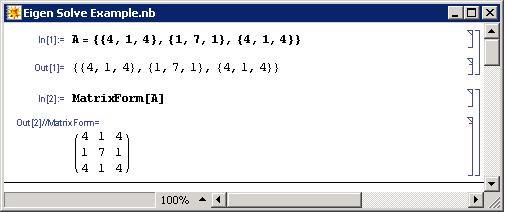
For larger matrices (4x4 and larger), solving for the eigenvalues and eigenvectors becomes very lengthy. Therefore software programs like Mathematica are used. The example from the last section will be used to demonstrate how to use Mathematica. First we can generate the matrix A. This is done using the following syntax:
- \(A = \{\{4,1,4\},\{1,7,1\},\{4,1,4\}\}\)
It can be seen that the matrix is treated as a list of rows. Elements in the same row are contained in a single set of brackets and separated by commas. The set of rows are also contained in a set of brackets and are separated by commas. A screenshot of this is seen below. (Note: The "MatrixForm[]" command is used to display the matrix in its standard form. Also in Mathematica you must hit Shift + Enter to get an output.)
Next we find the determinant of matrix A-λI, by first subtracting the matrix λI from A (Note: This new matrix, A-λI, has been called A2).
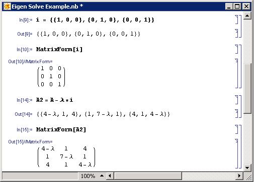
The command to find the determinant of a matrix A is:
- Det[A]
For our example the result is seen below. By setting this equation to 0 and solving for λ, the eigenvalues are found. The Solve[] function is used to do this. Notice in the syntax that the use of two equal signs (==) is used to show equivalence whereas a single equal sign is used for defining a variable.
- Solve[{set of equations},{variables being solved}]

Alternatively the eigenvalues of a matrix A can be solved with the Mathematica Eigenvalue[] function:
- Eigenvalues[A]
Note that the same results are obtained for both methods.

To find the eigenvectors of a matrix A, the Eigenvector[] function can be used with the syntax below.
- Eigenvectors[A]
The eigenvectors are given in order of descending eigenvalues.

One more function that is useful for finding eigenvalues and eigenvectors is Eigensystem[]. This function is called with the following syntax.
- Eigensystem[A]
In this function, the first set of numbers are the eigenvalues, followed by the sets of eigenvectors in the same order as their corresponding eigenvalues.

The Mathematica file used to solve the example can be found at this link.Media:Eigen Solve Example.nb
Microsoft Excel
Microsoft Excel is capable of solving for Eigenvalues of symmetric matrices using its Goal Seek function. A symmetric matrix is a square matrix that is equal to its transpose and always has real, not complex, numbers for Eigenvalues. In many cases, complex Eigenvalues cannot be found using Excel. Goal Seek can be used because finding the Eigenvalue of a symmetric matrix is analogous to finding the root of a polynomial equation. The following procedure describes how to calculate the Eigenvalue of a symmetric matrix in the Mathematica tutorial using MS Excel.
(1) Input the values displayed below for matrix A then click menu INSERT-NAME-DEFINE “matrix_A” to name the matrix.
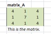
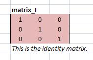
(2) Similarly, define identity matrix I by entering the values displayed below then naming it “matrix_I.”
(3) Enter an initial guess for the Eigenvalue then name it “lambda.”

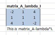
(4) In an empty cell, type the formula =matrix_A-lambda*matrix_I. Highlight three cells to the right and down, press F2, then press CRTL+SHIFT+ENTER. Name this matrix “matrix_A_lambda_I.”
(5) In another cell, enter the formula =MDETERM(matrix_A_lambda_I). This is the determinant formula for matrix_A_lambda_I.

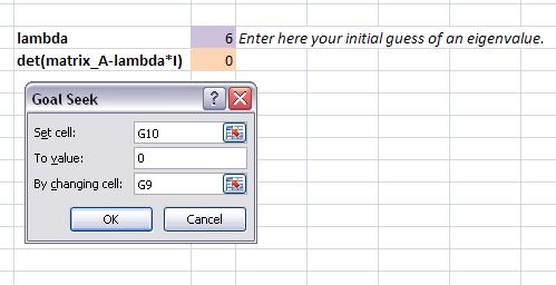
(6) Click menu Tools-Goal Seek… and set the cell containing the determinant formula to zero by changing the cell containing lambda.
(7) To obtain all three Eigenvalues for matrix A, re-enter different initial guesses. Excel calculates the Eigenvalue nearest to the value of the initial guess. The Eigenvalues for matrix A were determined to be 0, 6, and 9. For instance, initial guesses of 1, 5, and 13 will lead to Eigenvalues of 0, 6, and 9, respectively.
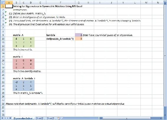
The MS Excel spreadsheet used to solve this problem, seen above, can be downloaded from this link: Media:ExcelSolveEigenvalue.xls.
Chemical Engineering Applications
The eigenvalue and eigenvector method of mathematical analysis is useful in many fields because it can be used to solve homogeneous linear systems of differential equations with constant coefficients. Furthermore, in chemical engineering many models are formed on the basis of systems of differential equations that are either linear or can be linearized and solved using the eigenvalue eigenvector method. In general, most ODEs can be linearized and therefore solved by this method. Linearizing ODEs For example, a PID control device can be modeled with ODEs that may be linearized where the eigenvalue eigenvector method can then be implemented. If we have a system that can be modeled with linear differential equations involving temperature, pressure, and concentration as they change with time, then the system can be solved using eigenvalues and eigenvectors:
\[\frac{d P}{d t}=4 P-4 T+C\nonumber \]
\[\frac{d T}{d t}=4 P-T+3 C\nonumber \]
\[\frac{d C}{d t}=P+5 T-C\nonumber \]
Note: This is not a real model and simply serves to introduce the eigenvalue and eigenvector method.
A is just the matrix that represents the coefficients in the above linear differential equations. However, when setting up the matrix, A, the order of coefficients matters and must remain consistent. Namely, in the following representative matrix, the first column corresponds to the coefficients of P, the second column to the coefficients of T, and the third column corresponds to the coefficients of C. The same goes for the rows. The first row corresponds to , the second row corresponds to
 , and the third row corresponds to
  :
:
\[\mathbf{A}=\left[\begin{array}{ccc}
4 & -4 & 1 \\
4 & -1 & 3 \\
1 & 5 & -1
\end{array}\right]\nonumber \]
It is noteworthy that matrix A is only filled with constants for a linear system of differential equations. This turns out to be the case because each matrix component is the partial differential of a variable (in this case P, T, or C). It is this partial differential that yields a constant for linear systems. Therefore, matrix A is really the Jacobian matrix for a linear differential system.
Now, we can rewrite the system of ODE's above in matrix form.

where
\[\mathbf{x}(t)=\left[\begin{array}{l}
P(t) \\
T(t) \\
C(t)
\end{array}\right]\nonumber \]
We guess trial solutions of the form
\[\mathbf{x}=\mathbf{v} e^{\lambda t}\nonumber \]
since when we substitute this solution into the matrix equation, we obtain
\[\lambda \mathbf{v} e^{\lambda t}=\mathbf{A} \mathbf{v} e^{\lambda t}\nonumber \]
After cancelling the nonzero scalar factor eλt, we obtain the desired eigenvalue problem.
\[\mathbf{A} \mathbf{v}=\lambda \mathbf{v}\nonumber \]
Thus, we have shown that
\[\mathbf{x}=\mathbf{v} e^{\lambda t}\nonumber \]
will be a nontrivial solution for the matrix equation as long as v is a nonzero vector and λ is a constant associated with v that satisfies the eigenvalue problem.
In order to solve for the eigenvalues and eigenvectors, we rearrange the Equation \ref{eq1} to obtain the following:
\[\left(\begin{array}{lllll}
\boldsymbol{\Lambda} & \lambda \mathbf{I}) \mathbf{v}=0 & & {\left[\begin{array}{ccc}
4-\lambda & -4 & 1 \\
4 & 1 & \lambda & 3 \\
1 & 5 & -1-\lambda
\end{array}\right] \cdot\left[\begin{array}{l}
x \\
y \\
z
\end{array}\right]=0}
\end{array}\right.\nonumber \]
For nontrivial solutions for v, the determinant of the eigenvalue matrix must equal zero, \(\operatorname{det}(\mathbf{A}-\lambda \mathbf{I})=0\). This allows us to solve for the eigenvalues, λ. You should get, after simplification, a third order polynomial, and therefore three eigenvalues. (see section on Solving for Eigenvalues and Eigenvectors for more details) Using the calculated eignvalues, one can determine the stability of the system when disturbed (see following section).
Once you have calculated the three eigenvalues, you are ready to find the corresponding eigenvectors. Plug the eigenvalues back into the equation  and solve for the corresponding eigenvectors. There should be three eigenvectors, since there were three eigenvalues. (see section on Calculating Eigenvalues and Eigenvectors for more details)
The solution will look like the following:
\[\left[\begin{array}{l}
P(t) \\
T(t) \\
C(t)
\end{array}\right]=c_{1}\left[\begin{array}{l}
x_{1} \\
y_{1} \\
z_{1}
\end{array}\right] e^{\lambda_{1} t}+c_{2}\left[\begin{array}{l}
x_{2} \\
y_{2} \\
z_{2}
\end{array}\right] e^{\lambda_{2} t}+c_{3}\left[\begin{array}{l}
x_{3} \\
y_{3} \\
z_{3}
\end{array}\right] e^{\lambda_{3} t}\nonumber \]
where
x1, x2, x3, y1, y2, y3, z1, z2, z3 are all constants from the three eigenvectors. The general solution is a linear combination of these three solution vectors because the original system of ODE's is homogeneous and linear. It is homogeneous because the derivative expressions have no cross terms, such as PC or TC, and no dependence on t. It is linear because the derivative operator is linear. To solve for c1, c2, c3 there must be some given initial conditions (see Worked out Example 1).
This Wiki does not deal with solving ODEs. It only deals with solving for the eigenvalues and eigenvectors. In Mathematica the Dsolve[] function can be used to bypass the calculations of eigenvalues and eigenvectors to give the solutions for the differentials directly. See Using eigenvalues and eigenvectors to find stability and solve ODEs for solving ODEs using the eigenvalues and eigenvectors method as well as with Mathematica.
This section was only meant to introduce the topic of eigenvalues and eigenvectors and does not deal with the mathematical details presented later in the article.
Using Eigenvalues to Determine Effects of Disturbing a System
Eigenvalues can help determine trends and solutions with a system of differential equations. Once the eigenvalues for a system are determined, the eigenvalues can be used to describe the system’s ability to return to steady-state if disturbed.
The simplest way to predict the behavior of a system if disturbed is to examine the signs of its eigenvalues. Negative eigenvalues will drive the system back to its steady-state value, while positive eigenvalues will drive it away. What happens if there are two eigenvalues present with opposite signs? How will the system respond to a disturbance in that case? In many situations, there will be one eigenvalue which has a much higher absolute value than the other corresponding eigenvalues for that system of differential equations. This is known as the “dominant eigenvalue”, and it will have the greatest effect on the system when it is disturbed. However, in the case that the eigenvalues are equal and opposite sign there is no dominant eigenvalue. In this case the constants from the initial conditions are used to determine the stability.
Another possible case within a system is when the eigenvalue is 0. When this occurs, the system will remain at the position to which it is disturbed, and will not be driven towards or away from its steady-state value. It is also possible for a system to have two identical eigenvalues. In this case the two identical eigenvalues produce only one eigenvector. Because of this, a situation can arise in which the eigenvalues don’t give the complete story of the system, and another method must be used to analyze it, such as the Routh Stability Analysis Method.
Eigenvalues can also be complex or pure imaginary numbers. If the system is disturbed and the eigenvalues are non-real number, oscillation will occur around the steady state value. If the eigenvalue is imaginary with no real part present, then the system will oscillate with constant amplitude around the steady-state value. If it is complex with a positive real part, then the system will oscillate with increasing amplitude around the function, driving the system further and further away from its steady-state value. Lastly, if the eigenvalue is a complex number with a negative real part, then the system will oscillate with decreasing amplitude until it eventually reaches its steady state value again.
Below is a table of eigenvalues and their effects on a differential system when disturbed. It should be noted that the eigenvalues developed for a system should be reviewed as a system rather than as individual values. That is to say, the effects listed in the table below do not fully represent how the system will respond. If you were to pretend that eigenvalues were nails on a Plinko board, knowing the location and angle of one of those nails would not allow you to predict or know how the Plinko disk would fall down the wall, because you wouldn't know the location or angle of the other nails. If you have information about all of the nails on the Plinko board, you could develop a prediction based on that information. More information on using eigenvalues for stability analysis can be seen here, Using eigenvalues and eigenvectors to find stability and solve ODEs_Wiki.


The above picture is of a plinko board with only one nail position known. Without knowing the position of the other nails, the Plinko disk's fall down the wall is unpredictable.

Knowing the placement of all of the nails on this Plinko board allows the player to know general patterns the disk might follow.
Repeated Eigenvalues
A final case of interest is repeated eigenvalues. While a system of \(N\) differential equations must also have \(N\) eigenvalues, these values may not always be distinct. For example, the system of equations:
\[\begin{align*}
&\frac{d C_{A}}{d t}=f_{A, in} \rho C_{A}=f_{out} \rho C_{A} \sqrt{V_{1}}-V_{1} k_{1} C_{A} C_{B}\\[4pt]
&\frac{d C_{B}}{d t}=f_{B, in} \rho C_{B in}-f_{out} \rho C_{B} \sqrt{V_{1}}-V_{1} k_{1} C_{A} C_{B}\\[4pt]
&\frac{d C_{C}}{d t}=-f_{out} \rho C_{c} \sqrt{V_{1}}+V_{1} k_{1} C_{A} C_{B}\\[4pt]
&\frac{d V_{1}}{d t}=f_{A, in}+f_{B, in}-f_{out} \sqrt{V_{1}}\\[4pt]
&\frac{d V_{2}}{d t}=f_{out} \sqrt{V_{1}}-f_{customer} \sqrt{V_{2}}\\[4pt]
&\frac{d C_{C 2}}{d t}=f_{\text {out}}, \rho C_{C} \sqrt{V_{1}}-f_{\text {customer}}, \rho C_{\mathrm{C} 2} \sqrt{V_{2}}
\end{align*} \nonumber \]
May yield the eigenvalues: {-82, -75, -75, -75, -0.66, -0.66}, in which the roots ‘-75’ and ‘-0.66’ appear multiple times. Repeat eigenvalues bear further scrutiny in any analysis because they might represent an edge case, where the system is operating at some extreme. In mathematical terms, this means that linearly independent eigenvectors cannot be generated to complete the matrix basis without further analysis. In “real-world” engineering terms, this means that a system at an edge case could distort or fail unexpectedly.
However, for the general solution:
\[Y(t)=k_{1} \exp (\lambda t) V_{1}+k_{2} \exp (\lambda t)\left(t V_{1}+V_{2}\right)\nonumber \]
If \(λ < 0\), as \(t\) approaches infinity, the solution approaches 0, indicating a stable sink, whereas if λ > 0, the solution approaches infinity in the limit, indicating an unstable source. Thus the rules above can be roughly applied to repeat eigenvalues, that the system is still likely stable if they are real and less than zero and likely unstable if they are real and positive. Nonetheless, one should be aware that unusual behavior is possible. This course will not concern itself with resultant behavior of repeat eigenvalues, but for further information, see:
- http://math.rwinters.com/S21b/supplements/newbasis.pdf
- http://www.sosmath.com/diffeq/system/linear/eigenvalue/repeated/repeated.html
Your immediate supervisor, senior engineer Captain Johnny Goonewadd, has brought you in on a project dealing with a new silcone-based sealant that is on the ground level of research. Your job is to characterize the thermal expansion of the sealant with time given a constant power supply. Luckily, you were given a series of differential equations that relate temperature and volume in terms of one another with respect to time (Note: T and V are both dimensionless numbers with respect to their corresponding values at t=0). Solve the system of differentials and determine the equations for both Temperature and Volume in terms of time.
Solution
You are given the initial condition at time t=0, T=1 and V=1
\[\frac{d T}{d t}=4 T-3 V\nonumber \]
\[\frac{d V}{d t}=3 T+4 V\nonumber \]
By defining a matrix for both the coefficients and dependant variables we are able to rewrite the above series of differentials in matrix form
\[A=\left[\begin{array}{cc}
4 & -3 \\
3 & 4
\end{array}\right]\nonumber \]
\[X=\left[\begin{array}{l}
T \\
V
\end{array}\right]\nonumber \]
\[A * X=\left[\begin{array}{l}
\frac{d T}{d V} \\
\frac{d V}{d t}
\end{array}\right]\nonumber \]
Lambda is inserted into the A matrix to determine the Eigenvalues


For each eigenvalue, we must find the eigenvector. Let us start with λ1 = 4 − 3i


Now we find the eigenvector for the eigenvalue λ2 = 4 + 3i


The general solution is in the form


A mathematical proof, Euler's formula, exists for transforming complex exponentials into functions of sin(t) and cos(t)

Thus

Simplifying

Since we already don't know the value of c1, let us make this equation simpler by making the following substitution


Thus, we get have our solution in terms of real numbers

Or, rewriting the solution in scalar form


Now that we have our solutions, we can use our initial conditions to find the constants c3 and c4
First initial condition: t=0, T=1


First initial condition: t=0, V=1


We have now arrived at our solution


See Using eigenvalues and eigenvectors to find stability and solve ODEs_Wiki for solving ODEs using the eigenvalues and eigenvectors.
Process Engineer, Dilbert Pickel, has started his first day for the Helman's Pickel Brine Factory. His first assignment is with a pre-startup team formulated to start up a new plant designed to make grousley sour pickle brine. Financial constraints have demanded that the process begin to produce good product as soon as possible. However, you are forced to reflux the process until you reach the set level of sourness. You have equations that relate all of the process variable in terms of one another with respect to time. Therefore, it is Dill Pickles job to characterize all of the process variables in terms of time (dimensionless Sourness, Acidity, and Water content; S, A, & W respectively). Below is the set of differentials that will be used to solve the equation.
\[\\begin{array}{l}
\frac{d S}{d t}=S+A+10 W \\
\frac{d A}{d t}=S+5 A+2 W \\
\frac{d W}{d t}=4 S+3 A+8 W
\end{array}]
Thus the coefficient matrix
\[\mathbf{A}=\left[\begin{array}{lll}
1 & 1 & 10 \\
1 & 5 & 2 \\
4 & 3 & 8
\end{array}\right]\nonumber \]
Using mathematica it is easy to input the coefficients of the system of equations into a matrix and determine both the eigenvalues and eigenvectors. 
The eigenvectors can then be used to determine the final solution to the system of differentials. Some data points will be necessary in order to determine the constants.
\[\left[\begin{array}{l}
S \\
A \\
W
\end{array}\right]=C_{1}\left[\begin{array}{c}
0.88 \\
0.38 \\
1
\end{array}\right] e^{(5+\sqrt{89} k}+C_{2}\left[\begin{array}{c}
2 \\
-4 \\
1
\end{array}\right] e^{4 t}+C_{3}\left[\begin{array}{c}
-2.74 \\
0.10 \\
1
\end{array}\right]\nonumber \]
See Using eigenvalues and eigenvectors to find stability and solve ODEs_Wiki for solving ODEs using the eigenvalues and eigenvectors.
It is possible to find the Eigenvalues of more complex systems than the ones shown above. Doing so, however, requires the use of advanced math manipulation software tools such as Mathematica. Using Mathematica, it is possible to solve the system of ODEs shown below.
\[\begin{aligned}
\frac{d X}{d t} &=8 X+\frac{10 X Y F}{X+Z} \\
\frac{d Y}{d t} &=4 F-Y-Z-\frac{3 X Y}{X+Y} \\
\frac{d Z}{d t} &=9 X-2 Z+F
\end{aligned}\nonumber \]
Obviously, this system of ODEs has 4 variables and only 3 equations.
Obviously, this is a more complex set of ODEs than the ones shown above. And even though they will create a more complex set of Eigenvalues, they are solved for in the same way when using Mathematica.
Using the code shown below:
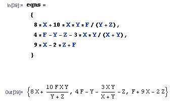
The equations can be entered into Mathematica. The equations are shown again in the output
Then, using the next bit of code:
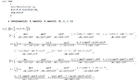
The it is possible to find where the equations are equal to 0 (i.e. the fixed points). The results of this is also shown in the image above. It's notable that 3 solutions are found. This makes sense as the system is 3 ODEs.
The Jacobian can then be found by simply using the code shown below.
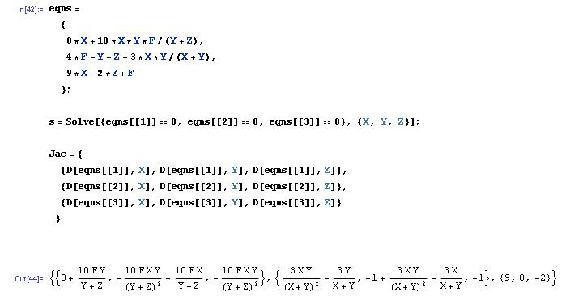
The ersults of finding the Jacobian are shown in the equation above.
Finally, to find one of the Eigenvalues, one can simply use the code shown below.
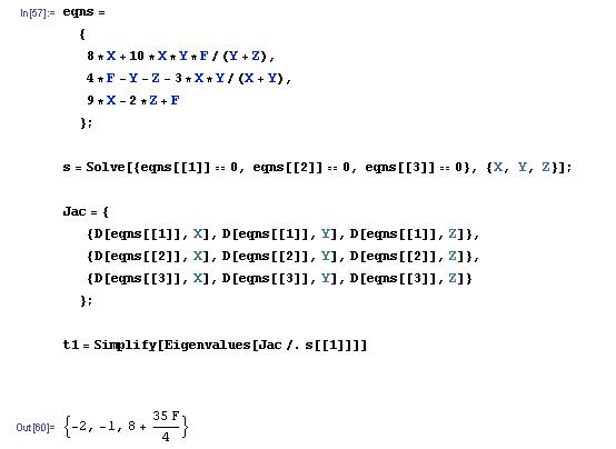
This gives the Eigenvalue when the first fixed point (the first solution found for "s") is applied. The other two solutions could be found by simply changing the fixed blade that is referred to when finding t1. The other Eigenvalues are not shown because of their large size.
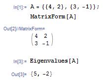
What are the eigenvalues for the matrix A?
\[\mathbf{A}=\left[\begin{array}{cc}
4 & 2 \\
3 & -1
\end{array}\right]\nonumber \]
- \(\lambda_{1}=-2\) and \(\lambda_{1}=5\)
- \(\lambda_{1}=2\) and \(\lambda_{1}=-5\)
- \(\lambda_{1}=2\) and \(\lambda_{1}=5\)
- \(\lambda_{1}=-2\) and \(\lambda_{1}=-5\)
- Answer
-
a.

When a differential system with a real negative eigenvalue is disturbed, the system is...
- Driven away from the steady state value
- Unchanged and remains at the disturbed value
- Driven back to the steady state value
- Unpredictable and the effects can not be determined
- Answer
-
c. A real negative eigenvalue is indicative of a stable system that will return to the steady state value after it is disturbed.
References
- Kravaris, Costas: Chemical Process Control: A Time-Domain Approach. Ann Arbor: The University of Michigan, pp 1-23, A.1-A.7.
- Bhatti, M. Asghar: Practical Optimization Methods with Mathematica Applications. Springer, pp 75-85, 677-691.
- Strang, Prof. Gilbert: “Eigenvalues and Eigenvectors.” Math 18.06. Lord Foundation of Massachusetts. Fall 1999.
- Edwards, C. Henry and David E. Penney: Differential Equations: Computing and Modeling. Upper Saddle River: Pearson Education, Inc, pp 299-365.
- Teknomo, Kardi. Finding Eigen Value of Symmetric matrix Using Microsoft Excel. http:\\people.revoledu.com\kardi\ tutorial\Excel\EigenValue.html
Contributors and Attributions
- Authors: (October 19, 2006) Tommy DiRaimondo, Rob Carr, Marc Palmer, Matt Pickvet
- Stewards: (October 22, 2007) Shoko Asei, Brian Byers, Alexander Eng, Nicholas James, Jeffrey Leto


