12.2: MIMO control using RGA
- Page ID
- 22517
Introduction
Single variable Input or Single variable Output (SISO) control schemes are just one type of control scheme that engineers in industry use to control their process. They may also use MIMO, which is a Multi-Input-Multi-Output control scheme. In MIMO, one or more manipulated variables can affect the interactions of controlled variables in a specific loop or all other control loops. A MIMO control scheme is important in systems that have multiple dependencies and multiple interactions between different variables- for example, in a distillation column, where a manipulated variable such as the reflux ratio could directly or indirectly affect the feed flow rate, the product composition, and the reboiler energy. Thus, understanding the dependence of different manipulated and controlled variables in a MIMO control scheme could be extremely helpful in designing and implementing a control scheme for a process.
One method for designing and analyzing a MIMO control scheme for a process in steady state is with a Relative Gain Array (RGA). RGA is useful for MIMO systems that can be decoupled (see the article about determining if a system can be decoupled). For systems that cannot be decoupled, model predictive control or neural networks are better choices of analysis tool than RGA. A good MIMO control scheme for a system that can be decoupled is one that can control a process variable without greatly affecting the other process variables. It must also be stable with respect to dynamic situations, load changes, and random disturbances. The RGA provides a quantitative approach to the analysis of the interactions between the controls and the output, and thus provides a method of pairing manipulated and controlled variables to generate a control scheme.
What is RGA?
Relative Gain Array is an analytical tool used to determine the optimal input-output variable pairings for a multi-input-multi-output (MIMO) system. In other words, the RGA is a normalized form of the gain matrix that describes the impact of each control variable on the output, relative to each control variable's impact on other variables. The process interaction of open-loop and closed-loop control systems are measured for all possible input-output variable pairings. A ratio of this open-loop 'gain' to this closed-loop 'gain' is determined and the results are displayed in a matrix.
\[R G A=\Lambda=\left[\begin{array}{cccc}
\lambda_{11} & \lambda_{12} & \cdots & \lambda_{1 n} \\
\lambda_{21} & \lambda_{22} & \cdots & \lambda_{2 n} \\
\vdots & & & \\
\lambda_{n 1} & \lambda_{n 2} & \cdots & \lambda_{n n}
\end{array}\right] \nonumber \]
The array will be a matrix with one column for each input variable and one row for each output variable in the MIMO system. This format allows a process engineer to easily compare the relative gains associated with each input-output variable pair, and ultimately to match the input and output variables that have the biggest effect on each other while also minimizing undesired side effects.
Understanding the Results of the RGA
- The closer the values in the RGA are to 1 the more decoupled the system is
- The maximum value in each row of the RGA determines which variables should be coupled or linked
- Also each row and each column should sum to 1
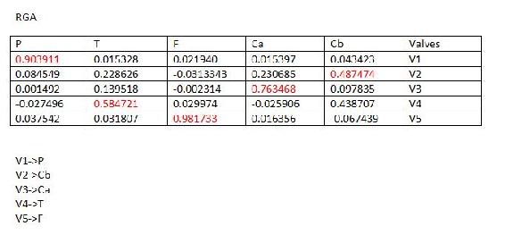
- Example
The table below includes the RGA results. The values highlighted in red are the maximum values in the row. These values indicated that the valve for that row should be used to control the variable that is listed in the corresponding column.
Calculating RGA
There are two main ways to calculate RGA:
- Experimentally determine the effect of input variables on the output variables, then compile the results into an RGA matrix.
- Use a steady-state gain matrix to calculate the RGA matrix.
Method (1) should be used when it is possible to carry out the experiments as detailed in the Calculating RGA with Experiments section. This method will generally yield the most accurate RGA matrix of the system because it is based on actual data taken from the operating control system. If performing these extensive experiments is not possible, method (2) can be used. If a process model is available, method (2) can be used with no experimental data. If there is no process model available, some experimental data must be taken (though less extensively than in method (1)) and used in conjunction with method (2).
Method 1: Calculating RGA with Experiments
This method of calculating the RGA can be used when it is possible to run experiments on each of the input-output pairings. Below is a step-by-step explanation of how to experimentally compile the RGA for a simple MIMO system.
The simplest MIMO system is one that has two inputs and two outputs. Remember that by definition, a change in one of the inputs in a MIMO system will change both of the outputs. This system can be expressed mathematically as written below.
\[y_1 = a_{11}m_1 + a_{12}m_2 \nonumber \]
\[y_2 = a_{21}m_1 + a_{22}m_2 \nonumber \]
Where yi is the output for loop i, the m variables are the inputs for each loop, and the a variables are the transfer functions. It also helps to see this system as a control diagram, as shown here.
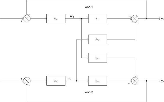
Clearly, both y1 and y2 are affected by both inputs (m1 and m2). Because of this, there are two choices for control. y1 could be controlled by m1, or y1 could be controlled by m2. y2 would then be controlled by the input that is not controlling y1. For a MIMO system with n input variables, there are n! possible control configurations. The question is: Which configuration will give you the best control? The answer can be determined by finding the relative gain array (RGA). There are a few ways to determine the RGA, one of which is by doing two experiments, repeated for every possible configuration. The RGA can be assembled from the data collected. These experiments are explained below using the above drawing and the configuration where m1 controls y1.
Experiment 1
For the first experiment, the objective is to observe the effect of m1 on y1. To do this, all of the loops must be open. In other words, the feedback loop is removed and the system is run manually with no control. This configuration is shown below.
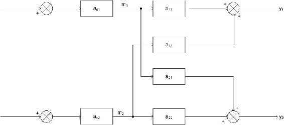
Now, since the system is under manual control, it is possible to introduce a step change Δm1 while keeping m2 constant. Because m2 is held constant, the change in y1, Δy1, can be attributed entirely to m1. Although a change in m1 will also affect y2, it is the relationship between m1 and y1 that must be observed at this point. Then, the gain of y1 with respect to m1 with all loops open is defined as g11. The calculation of g11 is shown below.
\[g_{11}=\frac{\Delta y_{1}(\text { all - loops -open })}{\Delta m_{1}(\text { all }-\text { loops -open })} \nonumber \]
The final objective of experiment one is obtaining the value gij where the controlled variable i is controlled by manipulated variable j.
Experiment 2
The goal of experiment two is to determine the effect of m2 on y1. To do this, loop 1 must remain open, but all other loops remain closed. This configuration is shown below.
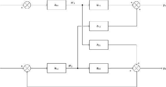
Now, the same step change that was introduced to m1 in experiment one must be introduced again. The difference is, now loop 2 is in perfect control which means that when m1 changes, it affects y2, so the control loop on loop two will adjust m2 in order to compensate and keep y2 constant. When m2 changes it, in turn, affects y1. It is this change that is being observed. The amount y1 changes is Δy1 and the amount m1 was stepped up is Δm1. Now:
\[g_{11}^{*}=\frac{\Delta y_{1}(\text { only }-\text { loop }-\text { one }-\text { open })}{\Delta m_{1}(\text { only }-\text { loop }-\text { one }-\text { open })} \nonumber \]
The objective of experiment two is to obtain this value of \(g_{i j}^{*}\) where controlled variable i is being controlled by manipulated j.
Compiling the Array
Once the experiments are run for every possible configuration, the results can be used to compile the relative gain array (RGA). To do this, we first have to find the relative gain. The relative gain is the ratio of  to
to  and is represented by
  .
.
\[\lambda_{i j}=\frac{g_{i j}}{g_{i j}^{*}}=\frac{\left(\frac{\delta y_{i}}{\delta m_{j}}\right)_{\text {all-loops-open }}}{\left(\frac{\delta y_{i}}{\delta m_{j}}\right)_{\text {only-loop-i-open }}}\]
The value for λ must be computed for every possible combination of i and j. After every value is found, the RGA matrix can be formed:
\[R G A=\Lambda=\left[\begin{array}{cccc}
\lambda_{11} & \lambda_{12} & \cdots & \lambda_{1 n} \\
\lambda_{21} & \lambda_{22} & \cdots & \lambda_{2 n} \\
\vdots & & & \\
\lambda_{n 1} & \lambda_{n 2} & \cdots & \lambda_{n n}
\end{array}\right]\]
Method 2: Calculating RGA with Steady-State Gain Matrix
Sometimes it is not convenient or possible to perform the experiments described above on every control pairing possibility in the system. If that is the case, a steady-state gain matrix can be used to determine the RGA. If a process model is available, the steady-state gain matrix can be calculated from the model equations. If a process model is not available, the steady-state gain matrix can be calculated from experimental data (fewer experiments are required than when the RGA is calculated directly from experimental data as above). Once the steady-state gain matrix is calculated, it can be used to compute the RGA. Beware that a RGA has to have the same number of controlled variables and manipulated variables (same number of inputs and outputs) to be in an m x m matrix form.
Process Model Available
If a process model is available, the steady-state gain matrix relates the manipulated variables to the controlled variables according to the following equation:
\[\mathbf{y}=G \mathbf{m} \nonumber \]
where \(\mathbf{y}\) is a vector of the controlled variables:
\[\mathbf{y}=\left[\begin{array}{c}
y_{1} \\
y_{2} \\
\vdots \\
y_{n}
\end{array}\right] \nonumber \]
\(\mathbf{m}\)is a vector of the manipulated variables:
\[\mathbf{m}=\left[\begin{array}{c}
m_{1} \\
m_{2} \\
\vdots \\
m_{n}
\end{array}\right] \nonumber \]
and G is the steady-state gain matrix:
\[G=\left[\begin{array}{cccc}
g_{11} & g_{12} & \cdots & g_{1 n} \\
g_{21} & g_{22} & \cdots & g_{2 n} \\
\vdots & & & \\
g_{n 1} & g_{n 2} & \cdots & g_{n n}
\end{array}\right] \nonumber \]
The values of gij are calculated by taking partial derivatives of the equations governing the controlled variables. Specifically:
\[g_{i j}=\frac{\partial y_{i}}{\partial m_{j}} \nonumber \]
During differentiation, hold constant all manipulated variables other than mj. To fill in matrix G with numerical values, simply substitute the appropriate steady state values for the process into the expressions derived from differentiation.
Now that the steady-state gain matrix has been found, the RGA can be calculated with just a little bit more math. However, now that you have the steady state gain matrix, this might be a good time to determine if your system can even be decoupled! See the article on singular value decomposition for methods to check this. Assuming SVD gives a condition number of less than about 50, we can proceed to calculation of the RGA. First, define a matrix R to be the transpose of the inverse of matrix G:
\[R=\left(G^{-1}\right)^{\mathrm{T}} \nonumber \]
The calculation of the inverse of a matrix is quite complicated for anything larger than a 2x2 matrix. Fortunately Mathematica will do this with the following command for a square matrix M:
Inverse[M]
The transpose of a matrix is when the rows become columns and the columns become rows. For a square matrix, this just means reflecting across the diagonal running from the top left to the bottom right corner of the matrix. The transpose can be found in Mathematica with the following command:
Transpose[M]
The RGA can now be obtained one element at a time according to this equation:
\[\lambda_{i j}=g_{i j} r_{i j} \nonumber \]
Note that this is not your usual matrix multiplication! Here you multiply corresponding elements of the G and R matrices to get the corresponding element of the RGA. This is the type of multiplication Mathematica does with the standard multiplication operator.
See Example 1 below for a worked-out RGA calculation using this approach.
Process Model Not Available
In case there is no process model available and it is not feasible to determine the RGA by carrying out both experiments necessary for full experimental determination, it still may be possible to develop a steady-state gain matrix experimentally which can then be used to derive the RGA. In this case, just carry out experiment 1 as described above to determine the elements of the steady-state gain matrix:
\[g_{i j}=\frac{\Delta y_{i}}{\Delta m_{j}} \nonumber \]
with all loops open.
Each element of the steady-state gain matrix can be determined this way, and then the RGA can be calculated from the steady-state gain matrix as shown in the previous section.
Interpreting the RGA
There are some important properties and guidelines in understanding and analyzing the RGA, and what the different values of the RGA mean:
1) All elements of the RGA across any row, or down any column will sum up to one:
\[\sum_{i=1}^{n} \lambda_{i j}=\sum_{j=1}^{n} \lambda_{i j}=1 \nonumber \]
This makes calculating the RGA easier because:
- in 2X2 case, only 1 element must be calculated to determine all elements
- in 3X3 case, only 4 elements must be calculated to determine all elements
and so on.
2) The λij calculated from steady-state matrix is dimensionless and unaffected by scaling.
3) Each of the rows in the RGA represent one of the outputs. Each of the columns represent a manipulated variable.
- If λij = 0: The manipulated variable (mj) will have no effect on the output or the controlled variable (yi).
- If λij = 1: The manipulated variable mj affects the output yi without any interaction from the other control loops in the system. From the definition of λij, this implies that the gain loop with all loops open is equal to the gain loop with all other loops closed, ie: g11 = g*11.
- If λij < 0: The system will be unstable whenever mj is paired with yi, and the opposite response in the actual system may occur if other loops are opened in the system.
- If 0 < λij < 1: This implies that other control loops (mj- yi) are interacting with the manipulated and controlled variable control loop.
Three different relationships based on λ=0.5 imply different interpretations of pairing and the RGA:
- If λij = 0.5: The control pairing effect is equal to the retaliatory effect of other loops.
- If λij < 0.5: The other control loops are influencing the control pair, and the influence from the other control loops are greater than the influence from the control pair.
- If λij > 0.5: This means that the control pair has a greater influence on the system than the other control loops.
- If λij >1: The open-loop gain of the control pair is greater than the gain with all other loops closed, ie: g11 > g*11. The positive value of RGA indicates that the control pair is dominant in the system, but the other loops are still affecting the control pair in the opposite direction. The higher the value of λij, the more correctional effects the other control loops have on the pair.
| λij | Possible Pairing |
|---|---|
| λij = 0 | Avoid pairing mj with yi |
| λij = 1 | Pair mj with yi |
| λij < 0 | Avoid pairing mj with yi |
| λij = or < 0.5 | Avoid pairing mj with yi |
| λij >1 | Pair mj with yi |
Analysis with RGA
The Niederlinski Index (NI) is a calculation used to analyze the stability of the control loop pairings using the result of the RGA, evaluated at Steady State:
\[N I=\frac{|G|}{\prod_{i=1}^{n} g_{i i}} \nonumber \]
A negative NI value indicates instability in the control loop. For a 2  2 matrix, a positive NI value indicates stability in the pairings, but this is not necessarily true for larger matrices! For matrices larger than 2
  2, a conclusion can only be drawn from a negative NI, which indicates instability. NI should not be used for systems that have time delays (dead time), as the NI stability predictions assume immediate feedback to the controller. However, the index can be adapted for systems with dead time, although that application is beyond the scope of this article.
Here's an example NI calculation: given the steady state gain matrix
\[G=\left[\begin{array}{cc}
-0.002 & 0.001 \\
0.002 & 0.003
\end{array}\right] \nonumber \]
the NI can be calculated from the following expression:
\[N I=\frac{(-0.002 \times 0.003)-(0.001 \times 0.002)}{-0.002 \times 0.003}=1.333 \nonumber \]
Since this is a 2  2 matrix, the positive value of the NI indicates stability in the control loop pairings.
Optimizing a MIMO Control Scheme: Pairing Rules
The goal of the RGA and NI analysis is to quantitatively determine the optimal variable pairing for a given process. Some basic rules to remember when attempting to obtain an optimal pairing of control loops in a system are:
- Rule 1: The positive RGA elements that are closest to 1.0 should have the corresponding manipulated and controlled variables paired. When the CN number is large, implying a less decoupled system, one should look for the max RGA elements.
- Rule 2: If the NI value is negative, the loop pairing for that control system configuration is unacceptable.
A blending unit is used to dilute and cool down the product stream of a reactor. Three streams are combined in the mixer: the hot, concentrated stream from the reactor, a room temperature stream containing none of the product A, and a second room temperature stream containing some A produced elsewhere in the process. It is desired to control the flow rate, temperature, and concentration of A in the product stream by manipulating the flow rates of the three input streams. A schematic of the process follows, filled in with the steady state values of flow rate, temperature, and concentration. The manipulated variables are indicated with the letter m and the controlled variables are indicated with the letter y:
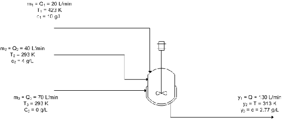
The equations used to model the system are:
\[y_{1}=m_{1}+m_{2}+m_{3} \nonumber \]
\[y_{2}=\frac{T_{1} m_{1}+T_{2} m_{2}+T_{3} m_{3}}{y_{1}}=\frac{T_{1} m_{1}+T_{2} m_{2}+T_{3} m_{3}}{m_{1}+m_{2}+m_{3}} \nonumber \]
\[y_{3}=\frac{c_{1} m_{1}+c_{2} m_{2}+c_{3} m_{3}}{y_{1}}=\frac{c_{1} m_{1}+c_{2} m_{2}+c_{3} m_{3}}{m_{1}+m_{2}+m_{3}} \nonumber \]
Calculate the RGA using the steady-state gain matrix method and use it to determine the best control scheme for the system.
Solution
First you must take the partial derivatives of the control variable equations in order to determine the elements of the steady-state gain matrix:
\[g_{11}=\frac{\partial y_{1}}{\partial m_{1}}=1 \nonumber \]
\[g_{21}=\frac{\partial y_{2}}{\partial m_{1}}=\frac{\left(T_{1}-T_{2}\right) m_{2}+\left(T_{1}-T_{3}\right) m_{3}}{\left(m_{1}+m_{2}+m_{3}\right)^{2}} \nonumber \]
\[g_{31}=\frac{\partial y_{3}}{\partial m_{1}}=\frac{\left(c_{1}-c_{2}\right) m_{2}+\left(c_{1}-c_{3}\right) m_{3}}{\left(m_{1}+m_{2}+m_{3}\right)^{2}} \nonumber \]
\[g_{12}=\frac{\partial y_{1}}{\partial m_{2}}=1 \nonumber \]
\[g_{22}=\frac{\partial y_{2}}{\partial m_{2}}=\frac{\left(T_{2}-T_{1}\right) m_{1}+\left(T_{2}-T_{3}\right) m_{3}}{\left(m_{1}+m_{2}+m_{3}\right)^{2}} \nonumber \]
\[g_{32}=\frac{\partial y_{3}}{\partial m_{2}}=\frac{\left(c_{2}-c_{1}\right) m_{1}+\left(c_{2}-c_{3}\right) m_{3}}{\left(m_{1}+m_{2}+m_{3}\right)^{2}} \nonumber \]
\[g_{13}=\frac{\partial y_{1}}{\partial m_{3}}=1 \nonumber \]
\[g_{23}=\frac{\partial y_{2}}{\partial m_{3}}=\frac{\left(T_{3}-T_{1}\right) m_{1}+\left(T_{3}-T_{2}\right) m_{2}}{\left(m_{1}+m_{2}+m_{3}\right)^{2}} \nonumber \]
\[g_{33}=\frac{\partial y_{3}}{\partial m_{3}}=\frac{\left(c_{3}-c_{1}\right) m_{1}+\left(c_{3}-c_{2}\right) m_{2}}{\left(m_{1}+m_{2}+m_{3}\right)^{2}} \nonumber \]
Now you can substitute in the given steady state values of the variables to find the numerical values of gij, obtaining:


In matrix form:
\[G=\left[\begin{array}{ccc}
1 & 1 & 1 \\
\frac{11}{13} & -\frac{2}{13} & -\frac{2}{13} \\
\frac{47}{845} & \frac{8}{845} & -\frac{18}{845}
\end{array}\right] \nonumber \]
Now calculate matrix R:
\[R=\left(G^{-1}\right)^{\mathrm{T}}=\left[\begin{array}{ccc}
\frac{2}{13} & \frac{4}{13} & \frac{7}{13} \\
1 & -\frac{5}{2} & \frac{3}{2} \\
0 & \frac{65}{2} & -\frac{65}{2}
\end{array}\right] \nonumber \]
You can now calculate the RGA by multiplying matrices G and R piecewise, according to the formula:
\[\lambda_{i j}=g_{i j} r_{i j} \nonumber \]
So the RGA is:
\[RGA=\left[\begin{array}{ccc}
\frac{2}{13} & \frac{4}{13} & \frac{7}{13} \\
\frac{11}{13} & \frac{5}{13} & -\frac{3}{13} \\
0 & \frac{4}{13} & \frac{9}{13}
\end{array}\right] \nonumber \]
Note that all rows and columns sum to 1, as they should.
Now it's time to determine the optimal control scheme for the system. The closer an element in the matrix is to 1, the better the pairing is between the manipulated and controlled variables represented by that element. With this in mind, we can immediately see that m1, the flow rate of stream 1, should be used to control y2, the temperature of the output stream, because the value of λ21 is the closest to 1 in the matrix ( ). Next in line is λ33, with a value of
  . This indicates that m3, the flow rate of stream 3, should control y3, the concentration of A in the product stream. So far so good, but what should control y1, the flow rate of the product stream? The best option would be m3, but this is already controlling the concentration of A in the product, so the next best option is m2, the flow rate of stream 2. This is not optimal because the relative gain is less than 0.5, but it is the best option available given the constraints of the system.
In a distillation column, reflux rate (R) and steam rate (S)are used to control the compositions in the distillate (xD)and the bottom product (xB). The control loops are opened in order to conduct experiment one as described above, and the following set of data is collected:
| Trial | R (kg/min) | S (kg/min) | xD | xB |
|---|---|---|---|---|
| 1 | 75 | 20 | 0.96 | 0.05 |
| 2 | 85 | 20 | 0.94 | 0.06 |
| 3 | 95 | 20 | 0.92 | 0.08 |
| 4 | 85 | 15 | 0.95 | 0.06 |
| 5 | 85 | 25 | 0.97 | 0.03 |
Calculate the RGA for this system, and determine which is the best pairing between the manipulated (R and S) and controlled variables (xD and xB).
Solution
From the experiment data, it is observed that the reflux rates (R) are constant for trials 2, 4 and 5, while the steam rates (S) are constant for trials 1, 2 and 3.
First, calculate the steady-state gain matrix for this system:
 with S constant
 with S constant
 with R constant
 with R constant
Organize the gain value into the matrix form and compute \(R\):
\[G=\left[\begin{array}{cc}
-0.002 & 0.001 \\
0.002 & 0.003
\end{array}\right] \nonumber \]
\[R=\left(G^{-1}\right)^{T}=\left[\begin{array}{cc}
-375 & 250 \\
125 & 250
\end{array}\right. \nonumber \]
Multiply each value in the R matrix by its corresponding gain value to obtain λij:
\[\lambda_{11}=g_{11} R_{11} \nonumber \]
\(λ_{ij}\) is then organized into the RGA matrix form:
\[R G A=\left[\begin{array}{cc}
\frac{3}{4} & \frac{1}{4} \\
\frac{1}{4} & \frac{3}{4}
\end{array}\right] \nonumber \]
The RGA matrix indicates that the composition of the distillate (xD) would be best controlled by the reflux flow (R); while xB would be best controlled by the steam rate (S)from the reboiler.
An example problem based from Fall 2008 second exam:
"Imagine that you are developing a control scheme for a new low temperature reactor system. The physics governing the system is complicated, so you decide to start out with an experiment on the system to see if you can develop a simple set if SISO controllers. To evaluate this possibility, you begin with your five valves at their steady state operating conditions (v1=0.5, v2=0.55, v3=0.5, v4=0.6, v5=0.4) and measure the five key variables of this process T1, T2, T3, P1 and P2. Next you slightly adjust each valve to see the steady state effects on each output variable"
As an approximation, you fit this model to the following system:
\[\left[\begin{array}{c}
T_{1} \\
T_{2} \\
T_{3} \\
P_{1} \\
P_{2}
\end{array}\right]=\left[\begin{array}{ccccc}
-0.2 & 0.06 & 0.03 & 1.0 & 0.02 \\
0.01 & 0.1 & -0.143 & 0.012 & 1.0 \\
0.5 & 1.0 & -0.23 & 0.04 & 0.02 \\
-0.2 & -0.1 & 1.0 & 0.123 & -0.023 \\
1.0 & -0.01 & 0.1 & 0.01556 & -0.013
\end{array}\right]\left[\begin{array}{c}
\mathrm{V}_{1} \\
\mathrm{v}_{2} \\
\mathrm{v}_{3} \\
\mathrm{v}_{4} \\
\mathrm{v}_{5}
\end{array}\right] \nonumber \]
"Perform an RGA analysis to find the best pairing between valves (v1, v2, v3, v4, and v5) and outputs (T1,T2, T3, P1, and P2)."
In Mathematica, you can input the matrix of coefficients by the following:

Note: I assign the matrix of coefficients to the variable, G.
It can be viewed in a matrix form in Mathematica by using function, "MatrixForm[]":
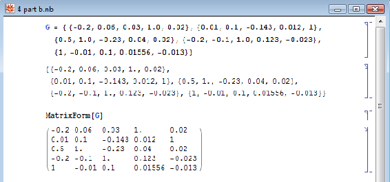
With the gain matrix, G, you can use the a singular value decomposition (SVD) of the gain matrix to determine how linearly dependent the model is. The linearity is based on the condition number (CN). Mathematica has a built-in function to do singular value decomposition. The following shows how to do singular value decomposition for this example.
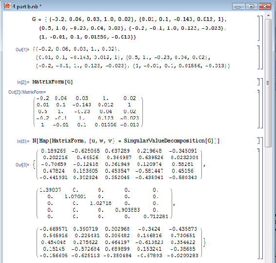
The Mathematica syntax is : N[Map[MatrixForm, {u, w, v} = SingularValueDecomposition[G]]]. The "SingularValueDecomposition[]" pops out three arrays assigned to variable u, w, and v . The "Map[MatrixForm, ..." portion pops out the three arrays into a matrix view and "N[.." portion forces numerical values in the matrices.
To the condition number(CN), you divide the biggest value by the smallest value in matrix, w. The general rule thumb is that if the condition number(CN) is greater than 50, then the system/model is too difficult to decouple.
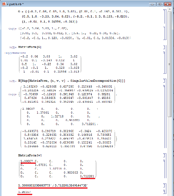
This illustrates that this system can be decoupled because the CN number is below 50. To determine the best pairing, RGA analysis is used in which it is a normalized form of the gain matrix, "G" that determines the impact of each control variable on its respective output e.g. how much impact does v1 have on T1, etc. The Mathematica syntax is N[G*Transpose[Inverse[G]]]. The RGA normalization is essential since at times, not in this case however, the values of the gain matrix may represent that a valve has great influence on multiple variables (ie. a column may contain the highest value from multiple rows). In order to distinguish unique separations between these influences, the RGA is used to normalize the gain matrix as seen below. This allows us to determine the different magnitudes of influence the valve has on an output in order to find the predominant effect on an output. The RGA illustrates these marginal differences in impact by the valves on the variable outputs, and lets us make the best possible pairings.

The best pairing is discovered by taking the maximum value of RGA Matrix for each row.

The bold values correspond to the valve that is the best pairing for the individual output. By looking at the bold values, V1->P2 V2->T3, V3-> P1, V4-> T1, V5-> T2.
For a MIMO control system containing 4 different manipulated and 4 different controlled variables, how many control configurations are possible for the system?
a. 24
b. 4
c. 64
d. 256
- Answer
-
a
Explanation: Mathematically, for an nxn manipulated by controlled variable system, the number of control configurations possible will be n! or n factorial. For a 4x4 variable system, 4x3x2x1 = 24. Physically, the number of control configurations translates to the number of possible input-output pairings.
In a case of a 2x2 matrix system, if one RGA element in first row calculated to be  . According to the RGA properties, what is the other element in that same row?
a. 
b. 
c. 
d. Cannot be determined with given information.
- Answer
-
b
Explanation: As explained above, all elements of the RGA across any row, or down any column should sum up to unity (one). For a 2x2 matrix, if one element in a row is
 , the other element must be 1-
 =
= 
RGA is useful for process engineers because it allows us to determine:
a. Which matrix size to use.
b. What eigenvalues and eigenvectors are paired.
c. What input and output pairs to use.
d. When feed forward control is preferred over feedback control.
- Answer
-
c
Explanation: Using RGA, a process engineer will assess the relative gain of pairing each input with each output to minimize undesired interactions and maximize desired interactions between controlled and manipulated variables in a system. See "Interpreting the RGA" section if you are confused on how this analysis is achieved.
References
- Berber, Ridvan. Methods of Model Based Process Control, Kluwer Academic Publishers, 1994.
- Lee, P.L., Newell, R.B., Cameron, I.T. Process Control and Management, Blackie Academic and Professional.
- Romagnoli, Jose A., Palazoglu, Ahmet. Introduction to Process Control, Taylor and Francis Group.
- Shinskey, F.G. Process Control Systems: Application, Design, and Tuning, Fourth Edition, McGraw-Hill, Inc., 1996.
- Svrcek, W.Y., Mahoney, D.P., and Young, B.R. A Real-Time Approach to Process Control, John Wiley and Sons, Ltd.
- Edinburgh University, Exercise: Relative Gain Arrays, 2006
- Edinburgh University, Multivariable Systems, 2007


