
3.3: Conservation of Mass Equation
- Page ID
- 81485

The recommended starting point for application of the conservation of mass equation is the rate-form of the mass balance (conservation of mass equation):
\[\frac{d m_{sys}}{d t} m= \sum_{in} \dot{m}_{i} - \sum_{out} \dot{m}_{e} \nonumber \]
where \(m_{sys}=\int_{V_{ms}} \rho \ dV\), the system mass, and \(\dot{m}\) is the mass flow rate across the system boundary.
In applying the rate-form of the conservation of mass equation to a system, there are many common modeling assumptions that can be used to set up the mathematical model of the physical system. These are detailed in the following paragraphs.
Steady-state system: For a steady-state system, all extensive and }}\) intensive properties are independent of time. Thus
\[\underbrace{\frac{d m_{sys}}{dt}}_{=0, \, \mathrm{SS}} = \sum_{in} \dot{m}_{i} - \sum_{out} \dot{m}_{e} \,\, \Rightarrow \,\, 0=\sum_{in} \dot{m}_{i}-\sum_{out} \dot{m}_{e} \nonumber \]
Incompressible substance: An incompressible substance is one for which the density never changes. Under these conditions, the mass flow rate can be written in terms of the density and the volumetric flow rate:
\[ \begin{align*} &\dot{m} = \int\limits_{A_c} \rho V_{rel, n} \ dA = \rho \int\limits_{A_c} V_{rel, n} \ dA \,\, \Rightarrow \,\, \dot{m} = \rho \dot{V\kern-0.8em\raise0.3ex-} \\ &m_{sys} = \int\limits_{V\kern-0.5em\raise0.3ex-_{sys}} \rho \ d V\kern-0.5em\raise0.3ex- = \rho \int\limits_{V\kern-0.8em\raise0.3ex-_{sys}} \,\, \Rightarrow \,\, m_{sys} = \rho V\kern-0.8em\raise0.3ex-_{sys} \end{align*} \nonumber \]
Although it is not a fundamental law, the following equation involving system volume and volumetric flow rates is often used to describe the behavior of systems.
\[ \frac{d V\kern-0.8em\raise0.3ex- _{sys}}{dt} = \sum_{in} \dot{ V\kern-0.8em\raise0.3ex-}_i - \sum_{out} \dot{ V\kern-0.8em\raise0.3ex-}_{e} : \nonumber \]
What conditions (or modeling assumptions) must apply for this equation to be valid? Try starting with Eq. \(\PageIndex{1}\) and deriving this equation for volume.
One-dimensional flow with uniform density at a flow boundary: Under these conditions both the density and the velocity come outside of the integral, giving
\[ \dot{m} = \int\limits_{A_c} \rho V_{rel, n} \ dA = \rho V_{rel, n} \int\limits_{A_c} dA \,\, \Rightarrow \,\, \dot{m} = \rho A_c V \nonumber \]
where velocity \(V\) used in calculating the mass flow rate is assumed to be the component of the velocity of the mass crossing the boundary that is normal to the boundary and measured relative to the boundary (regardless of whether the boundary is moving or stationary).
Please recognize that you should not concentrate on or memorize the final form of the equations developed above. Your focus should be on understanding the assumptions and learning how they impact the governing equations. As you will find later, the assumptions and their impact will be used repeatedly throughout these notes to help develop mathematical models for physical systems.
It is also sometimes required to apply the conservation of mass equation to a finite-time process when you are interested in relating what was known at some time \(t_1\) to some later time \(t_2\). Again, rather than memorizing a special form of the equation, just integrate the rate form of the conservation of mass equation as shown below:
\[\begin{align*} &\int\limits_{t_1}^{t_2} \left[ \frac{d m_{sys}}{dt} \right] \ dt = \int\limits_{t_1}^{t_2} \left[ \sum_{in} \dot{m}_i - \sum_{out} \dot{m}_e \right] \ dt \\[4pt] &\int\limits_{m_{sys, 1}}^{m_{sys, 2}} \ dm_{sys} = \int\limits_{t_1}^{t_2} \left( \sum_{in} \dot{m}_{i} \right) \ dt - \int\limits_{t_1}^{t_2} \left( \sum_{out} \dot{m}_{e} \right) \ dt \\[4pt] &m_{sys, 2} - m_{sys, 1} = \sum_{in} m_{i} - \sum_{out} m_{e} \end{align*} \nonumber \] where
\(m_{sys, 2}; \, m_{sys, 1} \, =\) mass inside the system at time \(t_2\) and \(t_1\), respectively.
\(m_{i} \equiv \int\limits_{t_1}^{t_2} \dot{m}_{i} \ dt \, =\) the amount of mass transported into the system during the time interval \(t_1\) to \(t_2\). (This is NOT the change in mass!)
The following examples demonstrate various applications of the conservation of mass equation to various problems.
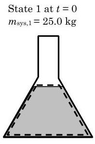
An open flask is filled with acetone. Initially, the flask contains \(25 \mathrm{~kg}\) of acetone. After two hours, some of the acetone evaporates and the flask contains \(23 \mathrm{~kg}\) of acetone. Taking your system to be the liquid acetone, answer the following questions by applying conservation of mass:
What is the accumulation of acetone during the two hours, in \(\mathrm{kg}\)?
How much acetone evaporated during the two hours, in \(\mathrm{kg}\)?
What is the average rate of evaporation during this time period, in \(\mathrm{kg} / \mathrm{s}\)?
Solution
Known: Acetone evaporates from an open flask
Find: Accumulation of the acetone, in \(\mathrm{kg}\).
Amount of acetone that evaporates, in \(\mathrm{kg}\).
Average rate of evaporation during this period, in \(\mathrm{kg} / \mathrm{h}\).
Given:
.jpg?revision=1)
Analysis:
Strategy \(\rightarrow\) What's the system? Liquid acetone as suggested in the problem statement.
What should we count? Mass of acetone.
What's the time period? Finite time period of 2 hours.
Selecting the liquid acetone as the system as shown in the figures above, we have an open system and there is only one interaction with the surrounding, the mass flow rate of acetone out of the system due to evaporation. This occurs at the free surface of the liquid in the flask.
Writing the rate form of the conservation of mass equation for this system we have
\[\frac{d m_{sys}}{dt} = \underbrace{ \cancel{ \sum_{in} \dot{m}_i } }_{\text {no inlet flows }}^{=0} \underbrace{ \cancel{ \sum_{out} \dot{m} i_e } }_{\text {only one outlet flow}} = \dot{m}_{\text {evap}} \quad \Rightarrow \quad \frac{d m_{\text {sys}}}{d t} = -\dot{m}_{\text {evap}} \nonumber \]
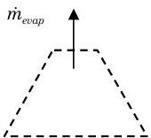
Figure \(\PageIndex{2}\): Rate of mass flow out of the system.
To find the accumulation, we must understand that the accumulation of the mass in the system is the change in the system mass
\[\Delta m_{sys} = m_{sys, 2} - m_{sys, 1} = (23.0 \mathrm{~kg})-(25.0 \mathrm{~kg})=-2.0 \mathrm{~kg} \nonumber \] Thus the accumulation of mass in the system is \(-2.0 \mathrm{~kg}\) of acetone.
To find the mass of acetone that has evaporated during these two hours, we must turn to the conservation of mass equation developed above. Since we want the amount of mass evaporated not the rate of evaporation, we must integrate the rate equation over the two-hour period.
\[\frac{d m_{sys}}{d t} = -\dot{m}_{evap} \quad \rightarrow \quad \int\limits_{t_1}^{t_2} \left( \frac{d m_{sys}}{d t} \right) \ dt = \int\limits_{t_1}^{t_2} \left( -\dot{m}_{evap} \right) \ dt \quad \rightarrow \quad \int\limits_{m_{sys,1}}^{m_{sys, 2}} dm_{sys} = -\int\limits_{t_1}^{t_2} \dot{m}_{evap} \ dt \quad \rightarrow \quad \Delta m_{sys} = -m_{evap} \nonumber \]
The left hand side just equals the accumulation of mass in the system and the right side is the amount of mass transported out of the system by mass transfer during the time interval. Thus the amount of mass evaporated is \[m_{evap} = -\Delta m_{sys} \quad \rightarrow \quad m_{evap} = -(-2.0 \mathrm{~kg}) = 2.0 \mathrm{~kg} \nonumber \]
Note that these two quantities could, in fact, be computed independently of each other with appropriate measurements. The connection between these quantities is the conservation of mass for this system.
To determine the average rate of evaporation, we can revisit the finite-time or integrated form of the conservation of mass equation
\[\frac{d m_{sys}}{dt} = -\dot{m}_{evap} \quad \rightarrow \quad \int\limits_{m_{sys, 1}}^{m_{sys, 2}} d m_{sys} = \underbrace{ -\int\limits_{t_1}^{t_2} \dot{m}_{evap} \ dt}_{\begin{array}{c} \text { assume mass flow } \\ \text { rate occurs at a } \\ \text{constant rate, } \dot{m}_{sys, evap} \end{array}} \quad \rightarrow \quad \Delta m_{sys} = -\dot{m}_{evap,avg} \Delta t \quad \rightarrow \quad \dot{m}_{evap, sys} = - \frac{\Delta m_{sys}}{\Delta t} \nonumber \]
Thus the average evaporation rate is
\[\dot{m}_{evap, avg} = -\frac{\Delta m_{sys}}{\Delta t} = -\frac{(-2.0 \ \mathrm{~kg})}{(2.0 \ \mathrm{hr})} = 1.0 \ \frac{\mathrm{kg}}{\mathrm{hr}} \nonumber \]
Comment:
Does the volume of the system change? If so what information would you need to be able to solve for the change in volume?
How would your solution change if you used a closed system that consisted of all of the acetone?
A hypodermic syringe is used to oil a machine part. The inside diameter of the glass syringe tube is \(1.0 \ \mathrm{cm}\) and the plunger moves inside the tube at the rate of \(0.5 \ \mathrm{~cm} / \mathrm{s}\). The syringe needle has an inside diameter of \(1.0 \ \mathrm{~mm}\). How long will it take to discharge \(12 \ \mathrm{cc}\) of oil? What is the velocity of the oil as it leaves the needle? (If necessary, you may assume that the oil is incompressible and the flow in the needle is one-dimensional.)
Solution
Known: A hypodermic syringe is used to oil parts.
Find: Volumetric flow rate of oil out of the needle, in \(\mathrm{cm}^3 / \mathrm{s}\).
Time required to discharge \(12 \ \mathrm{cc}\) of oil.
Velocity of the oil squirting out of the needle, in \(\mathrm{cm} / \mathrm{s}\).
Given:
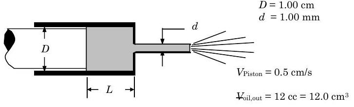
Figure \(\PageIndex{3}\): Setup of a syringe of oil, with the piston moving forward at a rate of \(0.5 \ \mathrm{cm/s}\).
Analysis
Strategy \(\rightarrow \quad\) System \(\rightarrow\) Volume occupied by oil inside the cylinder and needle
Property \(\rightarrow\) Count the mass of oil, since volume is related to mass.
Time interval \(\rightarrow\) Finite-time since amount of oil extruded given net rate.
Using the volume of oil inside the cylinder and needle as the open system, we can sketch a system diagram showing the mass flow rates.
Writing the conservation of mass equation for this system gives
\[ \frac{d m_{sys}}{dt} = \underbrace{ \cancel{ \sum_{in} \dot{m}_i }^{=0} }_{\begin{array}{c} \text{no inlets assuming} \\ \text{boundary at piston moves} \end{array}} - \underbrace{ \cancel{ \sum_{out} \dot{m}_e}^{= \dot{m}_{oil, out}} }_{\begin{array}{c} \text{one outlet assuming} \\ \text{no leakage at piston} \end{array}} \quad \rightarrow \quad \frac{d m_{sys}}{dt} = - \dot{m}_{oil, out} \nonumber \]
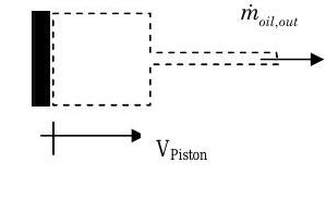
Figure \(\PageIndex{4}\): Velocity of piston motion and mass flow rate of oil out of the system.
Assuming uniform density for the oil gives \(m_{sys}=\rho_{oil} V\kern-0.8em\raise0.3ex- _{sys}\) and \(\dot{m}_{oil, out} = \rho_{oil} \dot{ V\kern-0.8em\raise0.3ex- }_{out} \).
Substituting these relations back into the conservation of mass equation, it becomes
\[ \frac{d m_{sys}}{d t} = -\dot{m}_{oil, out} \quad \rightarrow \quad \frac{d}{d t} \left( \rho_{oil} V\kern-0.8em\raise0.3ex- _{sys} \right) = -\rho_{oil} \dot{ V\kern-0.8em\raise0.3ex- }_{out} \quad \rightarrow \quad \cancel{ \rho_{oil} } \frac{d}{d t} \left( V\kern-0.8em\raise0.3ex- _{sys} \right) = - \cancel{ \rho_{oil} } \dot{ V\kern-0.8em\raise0.3ex- }_{out} \quad \rightarrow \quad \frac{d V\kern-0.8em\raise0.3ex- _{sys}}{d t} = -\dot{ V\kern-0.8em\raise0.3ex- }_{out} \nonumber \]
Note that for this particular problem, it appears that volume is conserved; however, in general this is not the case, or there would be a general law of conservation of volume.
Thinking about the volume of the system and that the boundary at the piston moves with the velocity \(V_{Piston}\), we can represent the rate of change of volume of the system in terms of the piston velocity and area as
\[\frac{d V\kern-0.8em\raise0.3ex- _{sys} }{d t} = -A_{Piston} V_{Piston} = -\left( \frac{\pi}{4} D^{2} \right) V_{Piston} \nonumber \] (Why do we have a minus sign?)
Now combining this with the result from the conservation of mass gives
\[\begin{align*} \frac{d V\kern-0.8em\raise0.3ex- _{sys}}{d t} &= -\dot{ V\kern-0.8em\raise0.3ex- }_{out} \\ -\left( \frac{\pi}{4} D^{2} \right) V_{Piston} &= -\dot{ V\kern-0.8em\raise0.3ex- }_{out} \quad \rightarrow \quad \dot{ V\kern-0.8em\raise0.3ex- }_{out} = \frac{\pi}{4} D^{2} V_{Piston} = \frac{\pi}{4} \left( 1.0 \ \mathrm{~cm}^{2} \right) \left( 0.5 \ \frac{\mathrm{cm}}{\mathrm{s}} \right) = 0.393 \ \frac{\mathrm{cm}^{3}}{\mathrm{~s}} \end{align*} \nonumber \]
Now to find the time needed to squirt \(12.0 \ \mathrm{~cm}^{3}\), we integrate the conservation of mass result
\[ \frac{d V\kern-0.8em\raise0.3ex- _{sys}}{dt} = - \dot{ V\kern-0.8em\raise0.3ex- }_{out} \quad \rightarrow \quad \int\limits_{ V\kern-0.5em\raise0.3ex- _{initial}}^{ V\kern-0.5em\raise0.3ex- _{final}} dV = - \int\limits_{t_{initial}}^{t_{final}} \dot{ V\kern-0.8em\raise0.3ex- }_{out} \ dt \quad \rightarrow \quad \Delta V\kern-0.8em\raise0.3ex- _{sys} = - \dot{ V\kern-0.8em\raise0.3ex- }_{out} \Delta t \nonumber \]
\[ \Delta t = \frac{\Delta V\kern-0.8em\raise0.3ex- _{sys}}{\dot{ V\kern-0.8em\raise0.3ex- }_{sys}} = \frac{ (12.0 \ \mathrm{cm}^3) }{\left( 0.393 \ \frac{\mathrm{cm}^3}{\mathrm{s}} \right)} = 30.5 \ \mathrm{seconds} \nonumber \]
Now to find the velocity of the oil leaving the needle, we can assume one-dimensional flow and use the definition of mass flow rate
\[\dot{ V\kern-0.8em\raise0.3ex- }_{out} = A_{out} V_{out} \quad \rightarrow \quad V_{out} = \frac{\dot{ V\kern-0.8em\raise0.3ex- }_{out}}{A_{out}} = \frac{\dot{ V\kern-0.8em\raise0.3ex- }_{out}}{\left( \frac{\pi}{4} D^{2} \right)} = \frac{\left( 0.393 \ \frac{\mathrm{cm}^{3}}{\mathrm{~s}} \right)}{\left( \frac{\pi}{4} \right)(0.1 \ \mathrm{~cm})^{2}}=50.0 \ \frac{\mathrm{cm}}{\mathrm{s}} \nonumber \]
Comment
Could you solve this problem with a non-deforming control volume? [Hint: Treat the piston entering the system as a mass flow rate. Then recognize that the mass in the system is changing.]
Could you solve this problem using a deforming, closed system? [Hint: Consider a closed, deforming system that includes all of the oil originally in the cylinder volume and the needle.]
Gasoline is pumped into a 1000 gallon storage tank at the rate of 10 gpm (gallons per minute). During the filling process, gasoline is being drained out at a rate of 2 gpm. The inlet and the drain are both located below the free surface of the gasoline in the tank. How long will it take to fill the tank if it initially contains 100 gallons of gasoline?
Solution
Known: Gasoline tank is being filled
Find: Time required to fill the tank.
Given:
.png?revision=1&size=bestfit&width=943&height=314)
Figure \(\PageIndex{5}\): Defining the system and the volumetric flow rates into and out of it.
Analysis:
Strategy \(\rightarrow \quad\) System \(\rightarrow\) Deforming volume of gasoline inside the tank during the entire process
Property to Count \(\rightarrow\) Mass of the oil
Time period \(\rightarrow\) Finite time
Writing conservation of mass for the deforming open system shown below, we have \[\frac{d m_{sys}}{d t}=\dot{m}_{1}-\dot{m}_{2} \nonumber \]
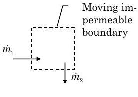
Figure \(\PageIndex{6}\): Gasoline in the tank forms a system with a moving impermeable boundary.
Assume uniform density and that the gasoline is incompressible, \(\dot{m}=\rho \dot{V\kern-0.8em\raise0.3ex-}\) and \(m=\rho V\kern-0.8em\raise0.3ex-\). Substituting these values back into the conservation of mass equation gives
\[\frac{d m_{sys}}{d t} = \dot{m}_1 - \dot{m}_2 \quad \rightarrow \quad \underbrace{ \frac{d}{d t} \left( \cancel{\rho} V\kern-0.8em\raise0.3ex-_{sys} \right) = \left( \cancel{\rho} \dot{V\kern-0.8em\raise0.3ex-}_1 \right) - \left( \cancel{\rho} \dot{V\kern-0.8em\raise0.3ex-}_2 \right) }_{\text{Density cancels out of all terms}} \quad \rightarrow \quad \frac{d V\kern-0.8em\raise0.3ex-_{sys}}{d t} = \dot{V\kern-0.8em\raise0.3ex-}_1-\dot{V\kern-0.8em\raise0.3ex-}_2 \nonumber \]
Now integrate with time to get the finite time form \[\int\limits_{t_i}^{t_f} \frac{d V\kern-0.8em\raise0.3ex-_{sys}}{d t} d t = \int\limits_{t_i}^{t_f} \left( \dot{V\kern-0.8em\raise0.3ex-}_1-\dot{V\kern-0.8em\raise0.3ex-}_2 \right) d t \quad \rightarrow \quad \Delta V\kern-0.8em\raise0.3ex- _{sys} = \underbrace{ \left(\dot{ V\kern-0.8em\raise0.3ex- }_1-\dot{ V\kern-0.8em\raise0.3ex- }_2 \right) \Delta t}_{\begin{array}{l} \text { Assumes that volumetric } \\ \text { flow rates are constant } \end{array}} \nonumber \]
Solving for the time interval \[\Delta t = \frac{\Delta V\kern-0.8em\raise0.3ex- _{sys}}{\left( \dot{ V\kern-0.8em\raise0.3ex- }_1-\dot{ V\kern-0.8em\raise0.3ex- }_2 \right)}=\frac{(1000-100) \ \cancel{\mathrm{gal}}}{(10-2) \frac{\cancel{\mathrm{gal}}}{\mathrm{min}}}=112.5 \ \mathrm {minutes} \nonumber \]
Comment
How would your answer change if \(\dot{V\kern-0.8em\raise0.3ex-}_2 = \left(2 \frac{\text {gal}}{\text{min}}\right) \left( \frac{t}{10 \ \text{min} +t}\right) \)?
Water flows steadily through a 3-inch diameter steel pipe before it passes through a reducer fitting into a 1-inch diameter pipe. All diameters are internal diameters. The average velocity in the larger pipe is 5 \(\mathrm{ft} / \mathrm{s}\). The density of water is \(62.4 \mathrm{lbm} / \mathrm{ft}^{3}\). Determine (a) the mass flow rate and the volumetric flow rate in the larger pipe, and (b) the volumetric flow rate and the average velocity in the smaller pipe.
Solution
Known: Water flows steadily through a reducer fitting
Find: Volumetric and mass flow rate in the 3-inch pipe. Volumetric flow rate and average velocity in 1-inch pipe.
Given:
.png?revision=1&size=bestfit&width=923&height=250)
Figure \(\PageIndex{7}\): Defining the system as the water within the reducer.
Strategy \(\rightarrow \quad \) System -- Non-deforming open system as shown in the figure to relate flows at the inlet and outlet.
Property to count -- Mass because we have to relate flows at two locations
Time period -- Steady-state problem since given only rates.
Writing the conservation of mass equation for this open system gives
\[ \underbrace{ \cancel{ \frac{d m_{sys}}{dt} }^{=0} }_{\begin{array}{c} \text {steady-state} \\ \text {conditions} \end{array}} =\dot{m}_{1}-\dot{m}_{2} \quad \rightarrow \quad \dot{m}_{2}=\dot{m}_{1} \nonumber \]
From the definition of average velocity \(\dot{m}=\rho A_{c} V_{\text {avg }}\) and \(\dot{V\kern-0.8em\raise0.3ex-}=A_{c} V_{\text {avg }}\) we can solve for the requested information at Inlet 1:
\[\begin{align*} &\dot{V\kern-0.8em\raise0.3ex-}_{1} = A_{c, 1} V_{avg, 1} = \left( \frac{\pi}{4} D_{1}^{2}\right) V_{avg, 1} = \left[ \frac{\pi}{4} \left(\frac{3.00}{12} \ \mathrm{ft}\right)^{2}\right] (5.00 \ \mathrm{ft} / \mathrm{s}) = 0.245 \ \frac{\mathrm{ft}^{3}}{\mathrm{~s}} \\ &\dot{m}_{1} = \rho \dot{V\kern-0.8em\raise0.3ex-}_{1} = \left(62.4 \ \frac{\mathrm{lbm}}{\mathrm{ft}^{3}}\right)\left(0.245 \ \frac{\mathrm{ft}^{3}}{\mathrm{~s}}\right) = 15.3 \ \frac{\mathrm{lbm}}{\mathrm{s}} \end{align*} \nonumber \]
Now at Outlet 2 we can make use of the conservation of mass results from above. Assuming that the density is uniform, then
\[\dot{m}_{2} = \dot{m}_{1} \quad \rightarrow \quad \cancel{ \rho } \dot{V\kern-0.8em\raise0.3ex-}_{2} = \cancel{ \rho } \dot{V\kern-0.8em\raise0.3ex-}_{1} \quad \rightarrow \quad \dot{V\kern-0.8em\raise0.3ex-}_{2} = 0.245 \ \frac{\mathrm{ft}^{3}}{\mathrm{~s}} \nonumber \]
To find the velocity \[\begin{align*} &\dot{V\kern-0.8em\raise0.3ex-}_{2}=\dot{V\kern-0.8em\raise0.3ex-}_{1} \quad \rightarrow \quad A_{c, 2} V_{avg, 2}=A_{c, 2} V_{c, 1} \quad \rightarrow \quad V_{avg, 2}=\frac{A_{c, 1}}{A_{c, 2}} V_{c, 1} \\ &V_{avg, 2} = \frac{\left(\dfrac{\pi}{4} D_{1}^{2}\right)}{\left(\dfrac{\pi}{4} D_{2}^{2}\right)} V_{avg, 1}=\left(\frac{D_{1}}{D_{2}}\right)^{2} V_{avg, 1}=\left(\frac{3}{1}\right)^{2} \left(5 \ \frac{\mathrm{ft}}{\mathrm{s}}\right) = 45.0 \ \frac{\mathrm{ft}}{\mathrm{s}} \end{align*} \nonumber \]
Consider the water tank shown below. The tank can be filled using either the tap at the top or the inlet at the bottom of the tank. The floor of the tank has an area of \(A_{\text {tank }}=10 \mathrm{~m}^{2}\), and the walls of the tank are vertical.
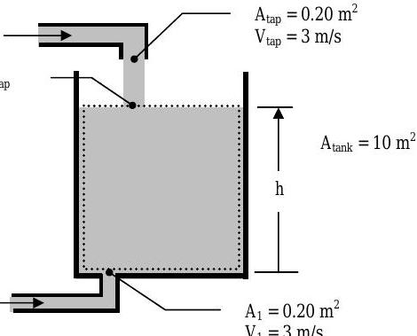
Figure \(\PageIndex{8}\): Defining the system and the two inlets leading into it.
The question at hand is, how long will it take to raise the level \(h\) of the water from 2 meters to 5 meters if I fill the tank with the inlet at the bottom of the tank? What if I use the tap at the top of the tank? Will it make any difference?
Filling the tank from the inlet in the floor of the tank
For purposes of this analysis, we must select a system, stuff to count, and a time period:
System \(\rightarrow\) Pick the volume of the water inside the tank. (See the dashed lines in the figure above. Mass can flow into this volume at 1 and the top boundary of the tank, which corresponds with the free surface of the water in the tank, moves up and down with the water. Call this System I.)
Stuff to count \(\rightarrow\) Mass of water inside the system
Time period \(\rightarrow\) Since we are asked to find the amount of time we will eventually need a finite-time analysis. (However, my experience, which I'm sharing with you, tells me that it is easiest to start with the rate-form (infinitesimal time period) and then integrate to get the finite-time form.)
Applying the conservation of mass equation to this system gives the following:
\[ \frac{d m_{sys}}{dt} = \dot{m}_1 \nonumber \]
Now to get the level or depth of the water into the problem, we need to consider how the mass of the system is related to the depth of the water. Applying the fundamental equation for calculating the mass inside a system gives the following result:
\[ m_{sys} = \int\limits_{V\kern-0.5em\raise0.3ex-_{sys}} \rho \ d V\kern-0.8em\raise0.3ex- = \underbrace{ \rho \int\limits_{V\kern-0.5em\raise0.3ex-_{sys}} d V\kern-0.8em\raise0.3ex- }_{\begin{array}{c} \text {Assume} \\ \text {uniform} \\ \text{density} \end{array}} = \rho V\kern-0.8em\raise0.3ex-_{sys} = \underbrace{ \rho A_{\text{tank}} h }_{\text{Since} V\kern-0.5em\raise0.3ex-_{sys} = A_{\text{tank}} h} \nonumber \]
Similarly, we need to determine the mass flow rate at 1 in terms of the known information as follows:
\[\dot{m}_{1} = \int\limits_{A_1} \rho V_{\text{n, rel}} \ dA = \underbrace{\rho_{1} \int_{A_1} V_{\text {n, rel}} \ dA}_{\begin{array}{c} \text { Uniform density} \\ \text {at the inlet} \end{array}} = \underbrace{\rho_1 V_1 \int\limits_{A_1} dA}_{\begin{array}{c} \text { Uniform velocity } \\ V_1=V_{\text{n, rel}} \end{array}} = \rho_{1} V_{1} A_{1} \nonumber \]
Now we can combine all of this information back into the conservation of mass equation Eq. \(\PageIndex{2}\) as follows:
\[\begin{align} \frac{d m_{sys}}{d t} &=\dot{m}_{1} \nonumber \\ \frac{d}{d t} \left( \rho A_{\text {tank}} h \right) &= \rho_{1} A_{1} V_{1} \end{align} \nonumber \]
Assuming that water is incompressible, then the density of water in the system \(\rho\) and the density of the water coming into the system \(\rho_{1}\) are the equal and the conservation of mass equation reduces (as developed in Eq. \(\PageIndex{5}\)) to
\[\begin{align} A_{\mathrm{tank}} \frac{d h}{d t} &=A_{1} V_{1} \nonumber \\ \frac{d h}{d t} &=\frac{A_{1}}{A_{\mathrm{tank}}} V_{1} \end{align} \nonumber \]
Integrating this equation to find the time it takes for \(h\) to go from 2 to 5 meters, we will use a definite integral between specified limits \[\begin{gather} \int d h = \int\left(\frac{A_1}{A_{\text{tank}}} V_1\right) dt = \left( \frac{A_1}{A_{\text{tank}}} V_1 \right) \int dt \quad \rightarrow \quad \int\limits_{h_1}^{h_2} dh=\int_{t_1}^{t_2} \left( \frac{A_1}{A_{\text{tank}}} V_1 \right) dt = \left(\frac{A_1}{A_{\text{tank}}} V_1 \right) \int\limits_{t_1}^{t_2} dt \nonumber \\ h_{2}-h_{1}=\left(\frac{A_{1}}{A_{\text {tank }}} V_{1}\right)\left(t_{2}-t_{1}\right) \end{gather} \nonumber \]
Now solving for the numerical answer we have
\[ \Delta t = t_2 - t_1 = \frac{\left( h_2 - h_1 \right) }{\left( \frac{A_1}{A_{\text{tank}} V_1} \right)} = \frac{(5-2) \ \mathrm{m}}{\left( \frac{0.2 \ \mathrm{m}^2}{10 \ \mathrm{m}^2} \right) \left( 3 \ \frac{\mathrm{m}}{\mathrm{s}} \right)} = 50 \ \mathrm{s} \nonumber \]
Filling the tank from the tap at the top of the tank
For purposes of this analysis, we must select a system, stuff to count, and a time period:
System \(\rightarrow\) Pick the volume of the water inside the tank. (See the dashed lines in the figure at below.) Mass can flow into this volume at 2, which is part of the upper boundary of the system. In addition, the entire top boundary of the tank, which corresponds with the free surface of the water in the tank, moves up and down with the water. Call this System II.
.png?revision=1&size=bestfit&width=730&height=531)
Figure \(\PageIndex{9}\): Defining the system and the two inlets leading into it.
Stuff to count \(\rightarrow\) Mass of water inside the system
Time period \(\rightarrow\) Since we are asked to find the amount of time, we will eventually need a finite-time analysis. (However, my experience, which I'm sharing with you, tells me that it is easiest to start with the rate-form (infinitesimal time period) and then integrate to get the finite-time form.)
Before you go on be sure you understand the difference between the system selected here (System II) and the one used previously (System I). This is very important.
Consider the questions:
- What is inside each system?
- Are they both open systems?
- Which boundaries have flow?
- Which boundaries move?
- How would you expect the shape of each system to change with time?
Applying the conservation of mass equation to System II gives the following:
\[ \frac{d m_{sys}}{dt} = \dot{m}_2 \nonumber \]
Now to get the level or depth of the water into the problem, we need to consider how the mass of the system is related to the depth of the water. Applying the fundamental equation for calculating the mass inside a system gives the following result:
\[ m_{sys} = \int\limits_{V\kern-0.5em\raise0.3ex-_{sys}} \rho \ d V\kern-0.8em\raise0.3ex- = \underbrace{ \rho \int\limits_{V\kern-0.5em\raise0.3ex-} d V\kern-0.8em\raise0.3ex- }_{\begin{array}{c} \text {Assume} \\ \text{uniform} \\ \text{density} \end{array}} = \rho V\kern-0.8em\raise0.3ex- = \underbrace{ \rho A_{\text{tank}} h }_{\text{Since } V\kern-0.5em\raise0.3ex-_{sys} = A_{\text{tank}} h} \nonumber \]
Similarly we need to determine the mass flow rate at inlet 2 in terms of the known information as follows:
\[ \dot{m}_2 = \int\limits_{A_2} \rho V_{\text{n, rel}} \ dA = \underbrace{ \rho_2 \int\limits_{A_2} V_{\text{n, rel}} \ dA }_{\begin{array}{c} \text{Uniform density} \\ \text{at the inlet} \end{array}} = \underbrace{ \rho_2 V_{\text{2, rel}} \int\limits_{A_2} dA }_{\begin{array}{c} \text {Uniform density} \\ V_{2, rel} = V_{n, rel} \end{array}} = \rho_2 V_{\text{2, rel}} dA = \rho V_{\text{2, rel}} A_2 \nonumber \]
At this point we must be very careful to correctly calculate the velocity of the mass crossing the system boundary. Recall that the mass flow rate is defined with respect to some boundary. For instance, the mass flow rate of the water leaving the tap, i.e., crossing the exit plane of the tap, is \(\dot{m}_{tap} = \rho A_{tap} V_{tap}\). This assumes that the density and velocity are uniform at the flow cross-section and that the velocity \(\mathbf{V_{tap}}\) is measured with respect to the exit plane of the tap.
Now, to calculate the mass flow rate at 2 on the boundary of our system requires that we know the velocity of the water relative to the system boundary that is moving.
.jpg?revision=1)
Figure \(\PageIndex{10}\): Rate of change of the upper system boundary.
Referring to the figure, we see that with respect to the ground (or any other stationary point) the velocity of the jet \(V_{tap}\) and the velocity of the boundary \(V_{boundary}\) can be sketched on the figure. The position of the boundary (the free surface of the water) can be defined in terms of the height of the surface \(h\) measured from the bottom of the tank. The velocity of the boundary with respect to the bottom of the tank (a stationary point) can be defined as \(V_{boundary} = dh/dt\).
To calculate the relative velocity of the fluid entering the system measured with respect to the moving boundary we must resort to basic physics relations for relative velocity calculations:
Given object \(A\) moving with velocity \(V_A\) measured with respect to a stationary point \(O\) and object \(B\) moving with velocity \(V_B\) measured with respect to the same stationary point \(O\), then
the relative velocity of \(A\) with respect to \(B\) is \( \mathbf{V}_{A/B} = \mathbf{V}_A – \mathbf{V}_B\) and
the relative velocity of \(B\) with respect to \(A\) is \(\mathbf{V}_{B/A} = \mathbf{V}_B – \mathbf{V}_A\).
Applying this result to our problem above gives the result that
\[ \begin{align} \mathbf{V}_{2, \text{rel}} &= \mathbf{ V _{tap/boundary} } \nonumber \\ &= \mathbf{V}_{\text{tap}} - \mathbf{V}_{\text{boundary}} \nonumber \\ V_{2, \text{rel}} \mathbf{i}_{\text{in}} &= V_{\text{tap}} \mathbf{i}_{\text{in}} - \left( - V_{\text{boundary}} \mathbf{i}_{\text{in}} \right) \\ &= \left( V_{\text{tap}} + V_{\text{boundary}} \right) \mathbf{i}_{\text{in}} \nonumber \\ V_{2, \text{rel}} &= V_{\text{tap}} + V_{\text{boundary}} = V_{\text{tap}} + \frac{dh}{dt} \nonumber \end{align} \nonumber \]
where \(\mathbf{i}_{\text{in}}\) is a unit vector pointing into the system (see the figure above of the moving boundary).
Note that Eq. \(\PageIndex{12}\) makes physical sense. The system boundary and the incoming water are both moving towards each other; thus, increasing the tap velocity or increasing the rate of change of \(h\) will both increase the relative velocity of the water crossing the system boundary measured with respect to the moving boundary.
Now combining these results with the conservation of mass equation gives \[\frac{d m_{\mathrm{sys}}}{d t}=\dot{m}_{2} \quad \rightarrow \quad \frac{d}{dt} \left( \rho A_{\mathrm{tank}} h \right) = \rho_{2} A_{2} V_{2, \mathrm{rel}} \quad \rightarrow \quad \frac{d}{dt} \left( \rho A_{\mathrm{tank}} h \right) = \rho_{2} A_{2} \left( V_{\mathrm{tap}} + \frac{d h}{d t} \right) \nonumber \]
Again assuming that water is an incompressible substance and also assuming that the area \(A_{2}=A_{\text {tap }}{ }^{1}\) gives us the following result:
\[\begin{gather} \frac{d}{d t}\left(\rho A_{\text {tank }} h\right)=\rho_{2} A_{2}\left(V_{\text {tap }}+\frac{d h}{d t}\right) \quad \rightarrow \quad \rho A_{\text {tank }} \frac{d h}{d t}=\rho_{2} A_{2}\left(V_{\text {tap }}+\frac{d h}{d t}\right) \nonumber \\ \left(A_{\text {tank }}-A_{2}\right) \frac{d h}{d t}=A_{2} V_{\text {tap }} \nonumber \\ \frac{d h}{d t}=\left(\frac{A_{2}}{A_{\text {tank }}-A_{2}}\right) V_{\text {tap }} \end{gather} \nonumber \]
Integrating Eq. \(\PageIndex{14}\) as before we obtain:
\[h_{2} - h_{1} = \left( \frac{A_2}}{A_{\text {tank}}-A_2} \right) V_{\text {tap}} \left( t_2-t_1 \right) \nonumber \]
And solving for the numerical answers, we obtain
\[\Delta t = t_2 -t_1 = \frac{ \left( h_2-h_1 \right) }{\left[ \left(\frac{A_2}{A_{\text {tank}}-A_2} \right) V_{\text {tap}} \right]}=\frac{(5-2) \ \mathrm{m}}{\left[ \left( \frac{0.2 \ \mathrm{~m}^{2}}{(10-0.2) \ \mathrm{m}^{2}} \right) \left( 3 \ \frac{\mathrm{m}}{\mathrm{s}} \right) \right]}=49 \ \mathrm{~s} \nonumber \]
Note: You should note that the assumption that \(A_{2}=A_{\text {tap}}\) is directly related to our assumption that the absolute velocity of the tap water jet at the boundary is the same as the velocity of the water leaving the tap \(V_{\text {tap}}\)
Comparing the results
Which arrangement "fills" the tank faster? Does this seem strange to you?
How would the comparison change if \(A_{\text{tap}} = A_1 = 1 \ \mathrm{m}^2\)? Would System II still be faster?
- System I:
- System II:
Suppose I started with an empty tank. Will it always take less time to "fill" the tank if I use a tap?