
3.5: Accounting of Chemical Species
- Page ID
- 82331

For many problems, it is essential to keep track of the individual chemical species — atoms or molecules. Examples of these include
- combustion processes, e.g. burning gasoline in air
- mixing processes, e.g. mixing water and antifreeze
- any process with chemical reactions
- preparation of solid solutions, e.g. doped silicon crystal
Although the total mass is always conserved, no such conservation law exists for chemical species in general.
Experimenting with Conservation of Mass
To see what happens when we try to account for individual chemical species, consider the steady-state chemical reactor in Figure \(\PageIndex{1}\). Compound \(A\) and compound \(B\) flow into the reactor and combine to produce compound \(C\).
.png?revision=1)
Figure \(\PageIndex{1}\): Steady-state chemical reactor
Writing the rate-form of the conservation of mass equation gives \[\frac{d m_{s y s}}{d t}=\dot{m}_1 + \dot{m}_2 - \dot{m}_3. \nonumber \] For steady-state operation the rate of change of mass inside the system is zero. Rearranging and solving for the mass flow rate at the outlet gives \[\dot{m}_3 = \dot{m}_1 + \dot{m}_2. \nonumber \] Now let's try writing a similar equation for just compound \(C\). Starting with the conservation of mass equation for only compound \(C\) we have
\[ \underbrace{ \frac{dm_{C,sys}}{dt} }_{\begin{array}{c} \text {Rate of change} \\ \text {of compound } C \\ \text {inside the system} \end{array}} = \underbrace{ \dot{m}_{C, 1} + \dot{m}_{C, 2} }_{\begin{array}{c} \text {Mass flow rate} \\ \text {of compound } C \\ \text {entering the system} \end{array}} - \underbrace{ \dot{m}_{C, 3} }_{\begin{array}{c} \text {Mass flow rate} \\ \text {of compound } C \\ \text {leaving the system} \end{array}} \nonumber \]
By definition, for a steady-state system the intensive and extensive properties of the system are independent of time. Thus, the rate-of-change term must be zero. We also know from our problem statement that only compounds \(A\) and \(B\) enter the system; thus, the mass flow rates of \(C\) at inlets 1 and 2 are identically zero. Putting this together gives the following result: \[0=0 + 0 - \dot{m}_{C, 3} \nonumber \] This result is inconsistent with our understanding of the physical situation. We know that compound \(C\) is leaving our steady-state reactor. Where is it coming from? A few moments of reflection might suggest that our experience tells us that compound \(C\) is being generated inside the system.
If we tried writing similar equations for compound \(A\) and compound \(B\), we would come up with the same physically inconsistent result. In this case, we might conclude that compound \(A\) and compound \(B\) are being consumed inside this system.
To remedy this inconsistency let's attempt to modify our mass balance to account for generation and consumption of individual chemical species. For our particular chemical reactor the equation might look like this for compound \(i\):
\[\underbrace{ \frac{d m_{i, sys}}{d t} }_{\begin{array}{c} \text {Rate of accumulation} \\ \text {of compound } i \\ \text {inside the system} \end{array}} = \underbrace{ \dot{m}_{i, 1} + \dot{m}_{i, 2} - \dot{m}_{i, 3}} _ {\begin{array}{c} \text {Transport rate of} \\ \text {compound } i \\ \text {across the} \\ \text {system boundary} \end{array}} + \underbrace{ \dot{m}_{i, \text { gen}}} _ {\begin{array}{c} \text {Generation rate} \\ \text {of compound } i \\ \text {inside the system} \end{array}} - \underbrace{ \dot{m}_{i, \text { cons}}} _ {\begin{array}{c} \text {Consumption rate} \\ \text {of compound } i \\ \text {inside the system} \end{array}} \nonumber \]
Writing this equation for each of the three compounds in our chemical reactor subject to the appropriate assumptions, e.g. steady-state operation and pure compounds at the three flow boundaries, gives
\[\begin{array}{ll} \text { Compound } A: & 0=\dot{m}_{A, 1} - 0 + 0 - \dot{m}_{A, \text { cons }} \\ \text { Compound } B: & 0=\dot{m}_{B, 1} - 0 + 0 - \dot{m}_{B, \text { cons }} \\ \text { Compound } C: & 0=0-\dot{m}_{C, 3} + \dot{m}_{C, \text{ gen}} - 0 \end{array} \nonumber \]
If we sum these three equations we obtain the following relationship: \[0 = \underbrace{ \left[ \dot{m}_{A, 1} + \dot{m}_{B, 2} - \dot{m}_{C, 3} \right] }_{ =0 \atop \begin{array}{c} \text {From conservation} \\ \text {of total mass} \end{array}} + \left[ \dot{m}_{C, \text{ gen}} - \dot{m}_{A, \text { cons}}-\dot{m}_{B, \text { cons}} \right] \nonumber \] Since the terms in the first brackets on the right-hand side satisfy the conservation of total mass equation written earlier, we are left with the conclusion that the terms in the second set of brackets must satisfy the following relationship:
\[ \underbrace{ \dot{m}_{C, \text{ gen}} }_{\begin{array}{c} \text {Generation rate} \\ \text {of compound } C \\ \text {inside the system} \end{array}} - \underbrace{ \dot{m}_{A, \text{ cons}} }_{\begin{array}{c} \text {Consumption rate} \\ \text {of compound } A \\ \text {inside the system} \end{array}} - \underbrace{ \dot{m}_{B, \text{ cons}} }_{\begin{array}{c} \text {Consumption rate} \\ \text {of compound } B \\ \text {inside the system} \end{array}} = 0 \nonumber \]
Examining this result, it would seem that this relationship is a direct consequence of the empirical fact that the total mass is conserved. In the next section we will write a general accounting statement for any chemical species in terms of both the species mass and the number of moles of the species.
Accounting Equation for Chemical Species
Building on the results of the last section and our experience with the accounting framework, we can write two different accounting or balance equations for any individual chemical species.
Mass Basis for Compound \(i\)
On a mass basis, the accounting equation is written in terms of the system mass, mass flow rates, and generation and consumption of mass of the specified compound:
\[\underbrace{ \frac{d m_{i, sys}}{d t} }_{\begin{array}{c} \text {Rate of accumulation} \\ \text { of mass } \\ \text {of Compound } i \\ \text {inside the system} \end{array}} = \underbrace{ \left[ \sum_{in} \dot{m}_{i, i} - \sum_{out} \dot{m}_{i, e} \right] }_{\begin{array}{c} \text {Net flow rate} \\ \text {of mass} \\ \text {of Compound } i \\ \text {into the system} \end{array}} + \underbrace{ \left[ \dot{m}_{i, gen} - \dot{m}_{i, cons} \right] }_{\begin{array}{c} \text {Net generation rate} \\ \text {of mass} \\ \text{of Compound } i \\ \text {inside the system} \end{array}} \nonumber \] where \[\begin{aligned} m_{i, sys} &= \int_{V_{sys}} \rho_{i} \ dV, \text {the mass of } i \text{ inside the system }(\mathrm{kg}) \\ \dot{m}_{i, i} ; \, \dot{m}_{i, e} &=\text {mass flow rate of } i \text{ into or out of the system }(\mathrm{kg} / \mathrm{s}) \\ \dot{m}_{i, gen} ; \, \dot{m}_{i, cons} &=\text {generation/consumption rate of } i \text{ inside the system }(\mathrm{kg} / \mathrm{s}) \end{aligned} \nonumber \]
Note that the generation and consumption terms are each identically zero unless there are chemical reactions in the system.
Molar Basis for Compound \(i\)
On a molar basis, the accounting equation is written in terms of the system moles, molar flow rates, and generation and consumption of moles of the specified compound: \[\underbrace{ \frac{d n_{i, sys}}{dt} }_{\begin{array}{c} \text {Rate of Accumulation} \\ \text {of moles} \\ \text {of Compound } i \\ \text {inside the system} \end{array}} = \underbrace{\left[ \sum_{in} \dot{n}_{i, i} - \sum_{out} \dot{n}_{i, e} \right] }_{\begin{array}{c} \text {Net molar flow rate} \\ \text {of Compound } i \\ \text {into the system} \end{array}} + \underbrace{ \left[ \dot{n}_{i, gen} - \dot{n}_{i, cons} \right] }_{\begin{array}{c} \text {Net generation rate} \\ \text {of moles} \\ \text {of Compound } i \\ \text {inside the system} \end{array}} \nonumber \] where \[\begin{aligned} n_{i, sys} &=\int_{V_{sys}} \bar{\rho}_{i} \ dV, \text { the number of moles of} i \text{ inside the system (kmol) } \\ \bar{\rho}_{i} &=\text {molar density of } i \left(\mathrm{kmol} / \mathrm{m}^{3}\right) \\ \dot{n}_{i, i} ; \, \dot{n}_{i, e}&=\text {molar flow rate of } i \text{ into or out of the system }(\mathrm{kmol} / \mathrm{s}) \\ \dot{n}_{i, gen} ; \, \dot{n}_{i, cons}&=\text {generation/consumption rate of moles of } i \text { inside the system } (\mathrm{kmol} / \mathrm{s}) \end{aligned} \nonumber \] Again, as with the mass basis equation, the generation and consumption terms are each identically zero unless there are chemical reactions in the system.
Application of Chemical Species Accounting
There are two broad classes of problems in which chemical species accounting are important:
- Systems without chemical reactions, and
- Systems with chemical reactions.
Systems Without Chemical Reactions
If a system has no chemical reactions, the first thing to recognize is that both the generation rate and the consumption rate terms for any compound are identically zero.
- If the chemical composition for the system is also constant (with time) and uniform (in space), the species accounting equations duplicate the conservation of mass equations and add nothing to our analysis.
- If the chemical composition is also time dependent and non-uniform, the species accounting equations may provide additional information that supplements the conservation of mass equations. Examples of this include problems involving mixing, separation, and distillation.
When applying both the conservation of mass and the species accounting equations, it is important to recognize how many independent equations can be written for a specific system.
For any non-reactive system, the maximum number of independent equations that can be obtained by applying the conservation of total mass and species accounting equals the number of independent species involved in the process
Try your hand at deciding how many independent equations can be written for the following steady-state systems:
(a) Tee in an air duct
- Inlet-1 \(\quad\) Air
- Outlet-2 \(\quad\) Air
- Outlet-3 \(\quad\) Air
(b) Air separation process
- Inlet-1 \(\quad\) Air composed of \(79 \% \mathrm{~N}_{2}\) and \(21 \% \mathrm{O}_{2}\) (molar analysis)
- Outlet-2 \(\quad\) Pure \(\mathrm{O}_{2}\)
- Outlet-3 \(\quad\) Pure \(\mathrm{N}_{2}\)
(c) Humidifier
- Inlet-1 \(\quad\) Air
- Inlet-2 \(\quad\) Water vapor
- Outlet-3 \(\quad\) Air-water vapor mixture
(d) Mixing chamber
- Inlet-1 Water vapor \(\left(\mathrm{H}_{2} \mathrm{O}\right)\)
- Inlet-2 \(\quad\) Carbon dioxide \(\left(\mathrm{CO}_{2}\right)\)
- Inlet-3 Air composed of \(79 \% \mathrm{~N}_{2}\) and \(21 \% \mathrm{O}_{2}\) (molar analysis)
- Outlet-4 Gaseous mixture of \(\mathrm{H}_{2} \mathrm{O}, \, \mathrm{CO}_{2}, \, \mathrm{N}_{2}\),\) and \(\mathrm{O}_{2}\)
(e) Distillation process
- Inlet-1: \(\quad\) Water-alcohol mixture with composition 1
- Outlet-2: \(\quad\) Water-alcohol mixture with composition 2
- Outlet-3: \(\quad\) Water-alcohol mixture with composition 3
The next two examples demonstrate how to use the species accounting equations to solve problems that do not involve chemical reactions.
Species Accounting — Problems without Chemical Reaction
Problems with changing composition can be separated into two groups: systems with chemical reaction and systems without chemical reaction. The focus of this subsection is systems without chemical reaction.
Species Accounting Equations
For systems without chemical reaction, the species accounting equations can be written without the generation/consumption terms. In terms of the mass of component \(j\), the species accounting equation becomes
\[\frac{d m_{j, sys}}{d t} = \sum_{in} \dot{m}_{j, i} - \sum_{out} \dot{m}_{j, e} + \cancel {\dot{m}_{j, gen}}^{=0} - \cancel {\dot{m}_{j, cons}}^{=0} \quad \rightarrow \quad \frac{d m_{j, sys}}{d t} = \sum_{in} \dot{m}_{j, i} - \sum_{out} \dot{m}_{j, e} \nonumber \] and in terms of the amount of substance \(j\) (moles of component \(j\)) the species accounting equation becomes
\[\frac{d n_{j, sys}}{d t} = \sum_{in} \dot{n}_{j, i} - \sum_{out} \dot{n}_{j, e} + \cancel{\dot{n}_{j, gen}}^{=0} - \cancel{\dot{n}_{j, cons}}^{=0} \quad \rightarrow \quad \frac{d n_{j, sys}}{d t} = \sum_{in} \dot{n}_{j, i} - \sum_{out} \dot{n}_{j, e} \nonumber \]
These equations can be written to keep track of any chemical component when studying the behavior of a system with changing composition and no chemical reactions. Examples of this type of problem involve the physical processes of mixing, separation, and distillation.
Given a system with \(N_{\text {comp}}\) chemical compounds, you can write a total of \(N_{\text {comp}}+1\) equations by applying conservation of total mass \(m\) and applying species accounting for each of the \(N_{\text {comp}}\) compounds. Unfortunately, only \(N_{\text {comp}}\) of these equations are independent. (This means that any \(N_{\text {comp}}\) of the available \(N_{\text {comp }}+1\) equations above can be combined by simple algebra to recover the remaining equation.)
Composition Equations
The composition of the mixture can always be described in terms of the mass fractions and mole fractions. For any system, one composition equation can be written for each flow stream, and an additional composition equation can be written to describe the contents of the system. For a steady-state system, the system composition equation is unnecessary.
Consider an open system with three components \(A,\) \(B\), and \(C\). For each inlet or outlet stream, say stream 1, we can relate the mass (or molar) flow rate of each component to the total flow rate at the inlet or outlet as shown below: \[\begin{array}{llll} \dot{m}_1 = \dot{m}_{A, 1} + \dot{m}_{B, 1} + \dot{m}_{C, 1} &= m f_{A, 1} \dot{m}_{1} + m f_{B, 1} \dot{m}_{1} + m f_{C, 1} \dot{m} & \rightarrow & 1=m f_{A, 1} + m f_{B, 1} + m f_{C, 1} \\ \dot{n}_1 = \dot{n}_{A, 1} + \dot{n}_{B, 1} + \dot{n}_{C, 1} &= n f_{A, 1} \dot{n}_{1} + n f_{B, 1} \dot{n}_{1} + n f_{C, 1} \dot{n}_{1} & \rightarrow & 1 = n f_{A, 1} + n f_{B, 1} + n f_{C, 1} \end{array} \nonumber \] For the contents of the system, the mass or amount of substance (moles) for each component can be written as shown below:
\[\begin{array} m_{sys} &= m_{A, sys} + m_{B, sys} + m_{C, sys} \\ &= m f_{A, sys} m_{sys} + m f_{B, sys} m_{sys} + m f_{C, sys} m_{sys} \quad \rightarrow \quad &1 = mf_{A, sys} + mf_{B, sys} + mf_{C, sys} \\ n_{sys} &= n_{A, sys} + n_{B, sys} + n_{C, sys} \\ &=n f_{A, sys} n_{sys} + n f_{B, sys} n_{sys} + n f_{C, sys} n_{sys} \quad \rightarrow \quad &1 = nf_{A, sys} + nf_{B, sys} + nf_{C, sys} \end{array} \nonumber \]
A specific chemical process requires a mixture of methanol, ethanol, and water at a mass flow rate of \(200 \mathrm{~kg} / \mathrm{h}\). The product stream is formed by using two streams each containing only two components. The known information about flow rates and composition for this steady-state mixing problem is shown in the table.
Using the information in the table and any additional assumptions, determine the unknown compositions and flow rates. [Note: No chemical reactions occur.]
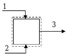
Figure \(\PageIndex{2}\): System setup for the mixing problem.
| Stream | Mass Flow Rate | Composition — Mass % | ||
| Methanol | Ethanol | Water | ||
| 1 | 0 | |||
| 2 | \(120 \mathrm{~kg} / \mathrm{h}\) | 0 | ||
| 3 | \(200 \mathrm{~kg} / \mathrm{h}\) | \(5.00\) | \(40.0\) | |
Analysis:
System \(\rightarrow\) See the picture
Time period \(\rightarrow\) Rate problem (Infinitesimal time difference)
Stuff to count \(\rightarrow\) Chemical species and mass.
There are 6 unknowns in this problem: one mass flow rate and five compositions. Thus we need 6 independent equations to relate these variables before we can solve the problem.
Apply conservation of mass and species accounting. Since there are 3 compounds we can obtain at most 3 independent equations by writing species accounting and conservation of mass equations for the system. Let’s write equations for total mass, ethanol and methanol:
\[ \begin{align*} \text{Mass Balance:} \quad \cancel{ \frac{d m_{sys}}{dt} }^{=0, SS} &= \dot{m}_1 + \dot{m}_2 - \dot{m}_3 \\ 0 &= \dot{m}_1 + \dot{m}_2 - \dot{m}_3 \end{align*} \nonumber \]
\[\begin{align*} \text{Ethanol Balance:} \quad \frac{d m_{\text{eth, sys}}}{d t} &= \dot{m}_{\text{eth, 1}} + \dot{m}_{\text {eth, 2}} - \dot{m}_{\text {eth, 3}} = m f_{\text {eth, 1}} \dot{m}_{1} + m f_{\text {eth, 2}} \dot{m}_{2} - m f_{\text {eth, 3}} \dot{m}_{3} \\ 0 &= m f_{\text {eth, 1}} \dot{m}_{1} + m f_{\text {eth, 2}} \dot{m}_{2} - m f_{\text {eth, 3}} \dot{m}_{3} \end{align*} \nonumber \]
\[\begin{align*} \text{Methanol Balance:} \quad \frac{d m_{\text {meth, sys}}}{d t} &= \dot{m}_{\text {meth, 1}} + \dot{m}_{\text {meth, 2}} -\dot{m}_{\text {meth, 3}} = m f_{\text {meth, 1}} \dot{m}_{1} + m f_{\text {meth, 2}} \dot{m}_{2} - m f_{\text {meth, 3}} \dot{m}_{3} \\ 0 &= m f_{\text {meth, 1}} \dot{m}_{1} + m f_{\text {meth, 2}} \dot{m}_{2} - m f_{\text {meth, 3}} \dot{m}_{3} \end{align*} \nonumber \]
Since we have used all of the independent species accounting or mass balance equations, we must now turn to the composition relations. There are three inlets/outlets, and so at most we can write 3 composition equations, one for each flow stream:
\[ \begin{align*} \text{Stream 1:} & \quad 1=m f_{\text{meth, 1}} + m f_{\text{eth, 1}} + m f_{\text{w, 1}} \\ \text{Stream 2:} &\quad 1=mf_{\text{meth, 2}} + m f_{\text{eth, 2}} + m f_{\text{w, 2}} \\ \text{Stream 3:} &\quad 1=m f_{\text{meth, 3}} + m f_{\text{eth, 3}} + m f_{\text{w, 3}} \end{align*} \nonumber \]
Since the problem is at steady-state, there is no need for a composition equation that describes the contents of the system.
We now have six equations that involve the six unknowns. Assuming that the equations are independent, we should be able to solve them for the unknowns. If we substitute the known information into the six equations, we have the following:
| \(0 = \dot{m}_1 + \dot{m}_2 - \dot{m}_3\) | \(\rightarrow\) | \(0 = \dot{m}_1 + \left( 120 \ \frac{\mathrm{kg}}{\mathrm{h}} \right) - \left( 200 \ \frac{\mathrm{kg}}{\mathrm{h}} \right)\) |
| \(0 = m f_{\text {eth, 1}} \dot{m}_{1} + m f_{\text {eth, 2}} \dot{m}_{2} - m f_{\text {eth, 3}} \dot{m}_{3}\) | \(\rightarrow\) | \(0 = (0) \dot{m}_1 + m f_{\text{eth, 2}} \left( 120 \ \frac{\mathrm{kg}}{\mathrm{h}} \right) - (0.40) \left( 200 \ \frac{\mathrm{kg}}{\mathrm{h}} \right)\) |
| \(0 = m f_{\text {meth, 1}} \dot{m}_{1} + m f_{\text {meth, 2}} \dot{m}_{2} - m f_{\text {meth, 3}} \dot{m}_{3}\) | \(\rightarrow\) | \( 0 = m f_{\text{meth, 1}} + (0) \left( 120 \ \frac{\mathrm{kg}}{\mathrm{h}} \right) - (0.05) \left( 200 \ \frac{\mathrm{kg}}{\mathrm{h}} \right) \) |
| \(1 = m f_{\text{meth, 1}} + m f_{\text{eth, 1}} + m f_{\text{w, 1}}\) | \(\rightarrow\) | \( 1 = m f_{\text{meth, 1}} + 0 + m f_{\text{w, 1}} \) |
| \(1 = m f_{\text{meth, 2}} + m f_{\text{eth, 2}} + m f_{\text{w, 2}}\) | \(\rightarrow\) | \( 1 = 0 + m f_{\text{eth, 2}} + m f_{\text{w, 2}} \) |
| \(1 = m f_{\text{meth, 3}} + m f_{\text{eth, 3}} + m f_{\text{w, 3}}\) | \(\rightarrow\) | \( 1 = 0.05 + 0.40 + m f_{\text{w, 3}} \) |
Solving these equations gives the following answers:
| Stream | Mass Flow Rate | Composition — Mass % | ||
| Methanol | Ethanol | Water | ||
| 1 | \( \mathbf{ 80 \ \mathrm{ \bf{kg}} / \mathrm{ \bf{h}} } \) | \(\bf{12.5}\) | \(0\) | \(\bf{87.5}\) |
| 2 | \( 120 \ \mathrm{kg} / \mathrm{h} \) | \(0\) | \(\bf{66.7}\) | \(\bf{33.3}\) |
| 3 | \(200 \ \mathrm{kg} / \mathrm{h} \) | \(5.00\) | \(40.0\) | \(\bf{55.0}\) |
This solution can be done by hand; however it is best done using a computer algebra system like MAPLE or a numerical solver like EES.
Lessons to be learned from this problem:
In general, for any problem with varying composition but no chemical reactions,
- each flow stream is specified by knowing its mass (or molar) flow rate and the mass (or mole) fractions of the components in the stream.
- the contents of each system are described by knowing the mass (or moles) and the composition of the contents.
- for each system (or subsystem), you can write one composition equation for each flow stream and one composition equation for the contents of the system. All of these equations are independent.
- for each system (or subsystem) in the problem, you can write as many independent mass and/or species accounting equations as there are chemical compounds (components) in the system (or subsystem).
For this example, there is one system with three flow streams and three compounds:
- Maximum number of variables to describe the compositions, mass, and flow rates:
\[(3 \text { mass flow rates})+(3 \text { flow streams})\left(3 \ \frac{\text {compounds}}{\text {flow stream}}\right)=12 \text { variables } \nonumber \]
- Maximum number of independent equations that can be written using composition, mass conservation, and species accounting:
\[\underbrace{(1 \text { system})(3 \text { compounds})}_{\begin{array}{c} \text { Number of independent total mass} \\ \text {and/or species accounting equations} \end{array}} + \underbrace{(3 \text { flow streams})}_{\begin{array}{c} \text {Number of independent} \\ \text {composition equations} \end{array}}=6 \text { independent equations} \nonumber \]
- The number of degrees of freedom is the difference between the number of variables needed to describe the problem and the number of independent equations you can write:
\[\underbrace{ \text{DOF}} _ {\begin{array}{c} \text {Degrees of} \\ \text {Freedom} \end{array}} = \underbrace{\text { NOV }}_{\begin{array}{c} \text {Number of} \\ \text {Variables} \end{array}} - \underbrace{\text {NOE}}_{\begin{array}{c} \text {Number of} \\ \text{Independent} \\ \text {Equations} \end{array}}= 12 - 6 = 6= \left[\begin{array}{c} \text {Minimum number of variables} \\ \text {that must be specified to obtain} \\ \text {a unique solution.} \end{array}\right] \nonumber \]
-
For this example, the problem statement provides information about six variables. Without this information it would have been impossible to find a unique solution.
If only five variables were assigned values, it would have only been possible to solve for 6 of the remaining variables in terms of the seventh variable. For example, if the mass flow rate at 2 had not been specified, you could have treated it as an independent variable and solved for all of the other unknown variables as a function of \(\dot{m}_{2}\). For a physically possible solution, \(\dot{m}_{2}\) could only take on a limited range of values, e.g. \(0<\dot{m}_{2}<200 \mathrm{~kg} / \mathrm{h}\) because stream 2 is the only way that ethanol is brought into the mixer.
With only five variables specified, a unique solution would only exist if additional constraints on the problem are provided. These could be provided in a number of ways - by specifying how some of the incoming mass or species flows must be distributed in the outlet, by giving you a range of compositions for certain variables, etc. These constraints serve as independent equations that can be combined with the independent equations developed from composition and species/mass accounting. This set can then be solved for the unknown variables.
If more than six variables were assigned values, not all of them could take on arbitrary values for the problem to have a solution.
A gas cylinder initially contains \(10 \ \mathrm{lbm}\) of air. It is desired to enrich the oxygen content of the mixture by bleeding \(5 \ \mathrm{lbm}\) of air from the cylinder and then adding \(3 \ \mathrm{lbm}\) of \(\mathrm{O}_{2}\). Determine the mass and molar composition of the mixture after the enrichment process is completed. For purposes of analysis you may assume that air is a mixture of \(23 \%\) oxygen and \(77 \%\) nitrogen by mass.
Solution
Known: Air is bled from a gas cylinder and replaced by oxygen.
Find: Composition (mass and mole fractions) after process
Given:
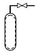
Figure \(\PageIndex{3}\): The system inside the tank.
\[ \begin{align*} \text{State 1:} \quad &m_{1}=10 \ \mathrm{lbm} \\ &m f_{\mathrm{O}_2}=0.23 ; \quad m f_{\mathrm{N}_2}=0.77 \end{align*} \nonumber \]
\[ \begin{align*} \text{Process 1} \rightarrow 2: \quad& \text{Remove } 5 \ \mathrm{lbm} \text{ air} \\ &\text{Add } 3 \ \mathrm{lbm} \text{ oxygen} \end{align*} \nonumber \]
Analysis:
Strategy \(\rightarrow\) To find compositions we must know the total mass and the mass of each component in the tank at the end of the enrichment process. If we can find the total mass and the mass of each component at the final state, we can answer this question. Thus, let's assume we have three unknowns. To solve for these we will apply an accounting equation since we want to relate the contents of a system at two different times.
System \(\rightarrow\) Treat the interior of the tank as a non-deforming open system.
Property \(\rightarrow\) Mass and chemical species
Time period \(\rightarrow\) Since only interest in initial and final states probably requires finite-time form
Writing the conservation of mass for any time during the enrichment process and then integrating over the time interval of the enrichment gives:
\[\frac{d m_{sys}}{d t} = \dot{m}_{in} - \dot{m}_{out} \quad \rightarrow \quad \int\limits_{t_1}^{t_2} \left( \frac{d m_{sys}}{d t} \right) dt = \int_{t_1}^{t_2} \left( \dot{m}_{in} - \dot{m}_{out} \right) dt \quad \rightarrow \quad m_{sys, 2}-m_{sys, 1} = m_{in}-m_{out } \nonumber \]
A similar expression can also be written for each chemical species in the problem: \[\begin{align*} \text{O}_{2}: \quad & \frac{d m_{sys, \text{O}_2}}{d t} = \dot{m}_{in, \ \text{O}_2} - \dot{m}_{out, \ \text{O}_2} & \rightarrow & m_{sys, \ \text{O}_2, \ 2} - m_{sys, \ \text{O}_2, \ 1} = m_{in, \ \text{O}_2} - m_{out, \ \text{O}_2} \\[4pt] \text{N}_{2}: \quad & \frac{d m_{sys, \ \text{N}_2}}{d t} = \dot{m}_{in, \ \text{N}_2} - \dot{m}_{out, \ \text{N}_2} & \rightarrow & m_{sys, \ \text{N}_2, \ 2} - m_{sys, \ \text{N}_2, \ 1} = m_{in, \ \text{N}_2} - m_{out, \ \text{N}_2} \end{align*} \nonumber \]
This gives three equations; however, only two of them are independent, i.e. the third equation can be formed by a linear combination of the other two equations.
To obtain the third independent equation, consider the composition in State 2 . This can be written in one of two forms:
\(\quad\) In terms of the actual mass we have \( \quad m_{sys, 2} = m_{sys, \text{O}_2, 2} + m_{sys, \text{N}_2, 2}\)
\(\quad\) In terms of the mass fractions we have \(\quad 1=m f_{sys, \text{O}_2, 2} + m f_{sys, \text{N}_2, 2}\)
As you can easily see, these two equations are not independent since the second equation is just the first equation divided through by the mass of the system.
Solving for the final mass \[m_{sys, \ 2}=m_{sys, \ 1} + m_{in} - m_{out} = (10+3-5) \ \mathrm{lbm} = 8 \ \mathrm{lbm} \nonumber \]
Now to find the amount of oxygen and nitrogen in the final state
m_{sys, \ \text{N}_2, \ 2} - m_{sys, \ \text{N}_2, \ 1} = \cancel{ m_{in, \ \text{N}_2} }^{=0} - m_{out, \ \text{N}_2}
m_{out, \ \text{N}_2} = m f_{out, \ \text{N}_2} \cdot m_{out} = (0.77) (5 \ \text{lbm}) = 3.85 \ \text{lbm} \quad \rightarrow \quad m_{sys, \ \text{N}_2, \ 2} = (7.70 - 3.85) \ \text{lbm} = 3.85 \ \text{lbm}
m_{sys, \ \text{N}_2, \ 1} = m f_{sys, \ \text{N}_2, \ 1} \cdot m_{sys, \ 1} = (0.77) (10 \ \text{lbm}) = 7.70 \ \text{lbm}
m_{sys, \ 2} = m_{sys, \ \text{N}_2, \ 2} + m_{sys, \ \text{O}_2, \ 2} \quad \rightarrow \quad
Now to find the compositions, use a simple table as below:
| \(\frac{m_{j}}{\mathrm{lbm}}\) | \(m f_{j}\) | \(\frac{M_{j}}{(\mathrm{lbm} / \mathrm{lbmol})}\) | \(\frac{n_{j}}{\mathrm{lbmol}}\) | \(n f_{j}\) | |
|---|---|---|---|---|---|
| \(\mathrm{O}_{2}\) | \(4.15\) | \(0.519\) | \(32.00\) | \(0.1297\) | \(0.485\) |
| \(\mathrm{N}_{2}\) | \(3.85\) | \(0.481\) | \(28.01\) | \(0.1375\) | \(0.515\) |
| \(8.00\) | \(1.000\) | \(\ldots \ldots\) | \(0.2672\) | \(1.000\) |
The weight percent of oxygen has increased from \(23 \%\) initially to a final value of \(51.9 \%\).
Comment:
Note that the mass fractions \((m f)\) and the mole fractions \((n f)\) are not the same. As indicated below the mass fraction indicates the composition in terms of the amount of mass of each component while the mole fraction only considers the number of molecules of the particles. \
[\begin{align*} m f & \rightarrow \frac{\text {mass of } j \text { molecules}}{\text {total mass of molecules}} \\ n f & \rightarrow \frac{\text {number of } j \text { molecules}}{\text {total number of molecules}} \end{align*} \nonumber \]
A liquid feed stream is fed continuously to a flash distillation chamber. As the liquid enters the chamber, its pressure is reduced and some of the entering liquid flashes to vapor. The liquid bottoms stream is drained from the floor of the chamber and the vapor distillate is removed near the top of the chamber.
The feed stream consists of water, ethanol, methanol entering at 25 \(\mathrm{lbm} / \mathrm{h}\), \(10 \mathrm{lbm} / \mathrm{h}\), and \(5 \mathrm{lbm} / \mathrm{h}\), respectively. The bottoms stream has a mass flow rate of \(24 \mathrm{lbm} / \mathrm{h}\) and consists of \(83.3 \%\) water, \(12.5 \%\) ethanol, and \(4.2 \%\) methanol by weight.
Determine the composition (mass and mole fractions) and the mass flow rate of the distillate.
Solution
Known: Operating conditions for a continuous flash distillation chamber.
Find: Composition (mass and mole fractions) and mass flow rate of the distillate.
Given:
.jpg?revision=1)
Figure \(\PageIndex{4}\): The system inside the flash chamber.
| Streams | |
|---|---|
| \(1- \text{Feed}\) |
\(\dot{m}_{\text {Water}}=25 \mathrm{lbm} / \mathrm{h}\) |
| \(2- \text{Distillate}\) | |
| \(3- \text{Bottoms}\) | \(m f_{\text {Water}}=83.3 \%\) \(m f_{\text {Ethanol}}=12.5 \%\) \(m f_{\text {Methanol}}=4.2 \%\) \(\dot{m}=24 \mathrm{lbm} / \mathrm{h}\) |
Analysis:
Strategy \(\rightarrow\) Since we are interested in relating entering flows to leaving flows, this seems like a candidate for conservation of mass and species accounting.
System \(\rightarrow\) Non-deforming, open system formed by the volume of the interior of the tank
Property \(\rightarrow\) Mass and species since we have mixtures which change composition
Time period \(\rightarrow\) Since system is fed continuously, assume steady-state
To completely specify all of the inlets and outlets of a problem like this requires knowing the composition and the total mass flow rate at each inlet/outlet OR the mass flow rate for each species and the total mass flow rate at each inlet/outlet. Thus the total number of unknowns is
\[ \underbrace{ \left[ \left( \text{Number of Species} \right) + 1 \right] }_{mf_{j} \text{'s and } \dot{m}} \times \left[ \text{Number of inlets/outlets} \right] = \left[ 3 \times 1 \right] \times \left[ 3 \right] = \underbrace{ 12 \ \text{unknowns} }_{\begin{array}{c} mf_{\text{Water}}, \ mf_{\text{Ethanol}}, \ mf_{\text{Methanol}}, \ \dot{m} \\ \text {for feed, distillate, and bottoms} \end{array}} \nonumber \]
\[ \underbrace{ \left[ \left( \text{Number of Species} \right) + 1 \right] }_{mf_{j} \text{'s and } \dot{m}} \times \left[ \text{Number of inlets/outlets} \right] = \left[ 3 \times 1 \right] \times \left[ 3 \right] = \underbrace{12 \text{ unknowns} }_ {\begin{array}{c} \dot{m}_{\text{Water}}, \ \dot{m}_{\text{Ethanol}}, \ \dot{m}_{\text{Methanol}} \\ \text {for feed, distillate, and bottoms} \end{array}} \nonumber \]
To help visualize what we know and don't know, set up a table:
| \(\dot{m}_{j} \ (\mathrm{lbm} / \mathrm{h}) \) | Composition | |||
|---|---|---|---|---|
| \(\text{Water}\) | \(\text{Ethanol}\) | \(\text{Methanol}\) | ||
| \(1 - \text{Feed}\) | \(\text{Eq. } 1\) | \(\text{Eq. } 2\) | \(\text{Eq. } 3\) | \(\text{Eq. } 4\) |
| \(2 - \text{Distillate}\) | \(\text{Eq. } 5\) | \(\text{Eq. } 6\) | \(\text{Eq. } 7\) | \(\text{Eq. } 8\) |
| \(3 - \text{Bottoms}\) | \(24.0\) | \(83.3\) | \(12.5\) | \(4.2\) |
By observing the table we see we already have four pieces of information. Given the mass flow rates at the feed stream we can find the composition at the feed stream using a feed stream composition relation \((\text{Eq. }1)\)
\[ \text{Eq. }1 \quad \rightarrow \quad \dot{m}_1 = \dot{m}_{\text {Water}, \ 1} + \dot{m}_{\text {Ethanol}, \ 1} + \dot{m}_{\text {Methanol}, \ 2} = (25+10+5) \ \frac{\mathrm{lbm}}{\mathrm{h}} = 40 \ \frac{\mathrm{lbm}}{\mathrm{h}} \nonumber \]
Then using the definition of mass fractions \((\text{Eq. } 2, \ 3,\) and \(4)\) for the feed stream:
\[ \text{Eq. } 2, \ 3, \ 4 \quad \rightarrow \quad m f_{\text {Water}, \ 1} = \frac{\dot{m}_{\text {water}, \ 1}}{\dot{m}_1} = \frac{25}{40} = 62.5 \% \ ; \quad m f_{\text {Ethanol}, \ 1} = \frac{10}{40}=25.0 \% \ ; \quad m f_{\text {Methanol}, \ 1} = \frac{5}{40}=12.5 \% \nonumber \]
Now there are only four unknowns remaining. The total mass flow rate can be solved for writing conservation of mass for the system \((\text{Eq. } 5)\)
\[ \text{Eq. } 5 \rightarrow \underbrace{ \cancel{ \frac{d m_{sys}}{dt} }^{=0} }_{\begin{array}{c} \text{steady-state} \\ \text{conditions} \end{array}} = \dot{m}_1 - \dot{m}_2 - \dot{m}_3 \quad \rightarrow \quad \dot{m}_2 = \dot{m}_1 - \dot{m}_3 = (40 - 24) \ \frac{\mathrm{lbm}}{\mathrm{h}} = 16 \ \frac{\mathrm{lbm}}{\mathrm{h}} \nonumber \]
The remaining unknowns can be determined by applying the species accounting equation for water, ethanol and methanol. The resulting equations look just like \(\text{Eq. } 5\) except they are written for each species.
\[ \begin{align*} &\dot{m}_{\text {water}, \ 2} = \dot{m}_{\text {water}, \ 1} - \dot{m}_{\text {water}, \ 3} = \dot{m}_{\text {water}, \ 1} - m f_{\text {water}, \ 3} \dot{m}_3 = [25.0 - (0.833)(24.0)] \ \frac{\mathrm{lbm}}{\mathrm{h}} = 5.01 \ \frac{\mathrm{lbm}}{\mathrm{h}} \\ &m f_{\text {water}, \ 2} = \frac{\dot{m}_{\text {water}, \ 2}}{\dot{m}_2} = \frac{5.01}{16.0} = 31.3 \% \end{align*} \nonumber \]
\[ \begin{align*} &\dot{m}_{\text {ethanol}, \ 2} = \dot{m}_{\text {ethanol}, \ 1} - \dot{m}_{\text {ethanol}, \ 3} = \dot{m}_{\text {ethanol}, \ 1} - m f_{\text {ethanol}, \ 3} \dot{m}_3 = [10.0-(0.125)(24.0)] \ \frac{\mathrm{lbm}}{\mathrm{h}} = 7.00 \ \frac{\mathrm{lbm}}{\mathrm{h}} \\ &m f_{\text {ethanol}, \ 2} = \frac{\dot{m}_{\text {ethanol}, \ 2}}{\dot{m}_2} = \frac{7.00}{16.0}=43.7 \% \end{align*} \nonumber \]
\[ \begin{align*} &\dot{m}_{\text {methanol}, \ 2} = \dot{m}_{\text {methanol}, \ 1} - \dot{m}_{\text {methanol}, \ 3} = \dot{m}_{\text {methanol}, \ 1} - m f_{\text {methanol}, \ 3} \dot{m}_{3} = [5.0-(0.042)(24.0)] \ \frac{\mathrm{lbm}}{\mathrm{h}} = 3.99 \ \frac{\mathrm{lbm}}{\mathrm{h}} \\ &m f_{\text {methanol}, \ 2} = \frac{\dot{m}_{\text {methanol}, \ 2}}{\dot{m}_2} = \frac{3.99}{16.0} = 25.0 \% \end{align*} \nonumber \]
The molar composition of the distillate can be computed after finding the molar flow rates:
| Mass flow rate | Molar mass | Molar flow rate | Mole fraction | |
|---|---|---|---|---|
| \(\text{Water}\) | \(5.01 \ \mathrm{lbm} / \mathrm{h}\) | \(18.02 \ \mathrm{lbm} / \mathrm{lbmol}\) | \(0.2780 \ \mathrm{lbmol} / \mathrm{h}\) | \(0.409\) |
| \(\text{Ethanol}\) | \(7.00 \ \mathrm{lbm} / \mathrm{h}\) | \(46.07 \ \mathrm{lbm} / \mathrm{lbmol}\) | \(0.1519 \ \mathrm{lbmol} / \mathrm{h}\) | \(0.224\) |
| \(\text{Methanol}\) | \(3.99 \ \mathrm{lbm} / \mathrm{h}\) | \(32.05 \ \mathrm{lbm} / \mathrm{lbmol}\) | \(0.2494 \ \mathrm{lbmol} / \mathrm{h}\) | \(0.367\) |
| \(16.00 \ \mathrm{lbm} / \mathrm{h}\) | \(\cdots\) | \(0.6793 \ \mathrm{lbmol} / \mathrm{h}\) | \(1.000\) |
Systems With Chemical Reactions
When chemical reactions occur in a system, the consumption and generation terms are no longer each zero. To evaluate these expressions, you must rely on the appropriate balanced chemical equations that apply to the reactions involved. Because of this, the molar form of the species accounting equation is the one commonly used when chemical reactions occur.
Again, it is important to recognize exactly how many independent equations can be obtained from applying conservation of mass and species accounting.
For a reactive system, the number of independent equations that can be obtained from conservation of mass and species accounting equals the number of independent species plus the number of independent chemical reactions. (The additional equations are supplied by the balanced chemical equations for each independent reaction.)
Applications for systems with chemical reactions are beyond the scope of this text. However, a brief example will illustrate how generation and consumption terms are obtained from the chemical equations. These topics are handled in greater detail in chemical engineering courses. The final example in this section demonstrates how a problem with chemical reactions could be approached.
A tank contains \(2 \ \mathrm{kmol}\) of carbon monoxide \((\mathrm{CO})\) and \(2 \ \mathrm{kmol}\) of oxygen \(\left(\mathrm{O}_{2}\right)\). If \(50 \%\) of the original amount of \(\mathrm{CO}\) is reacted with the \(\mathrm{O}_{2}\) to form \(\mathrm{CO}_{2}\), determine the amount of \(\mathrm{CO}, \mathrm{CO}_{2}\), and \(\mathrm{O}_{2}\) in the final mixture.
Solution
Known: A mixture of \(\mathrm{CO}\) and \(\mathrm{O}_{2}\) is reacted in a closed system.
Find: Amount of \(\mathrm{CO}, \mathrm{O}_{2}\), and \(\mathrm{CO}_{2}\) in mixture if \(50 \%\) of original \(\mathrm{CO}\) is reacted.
Given:
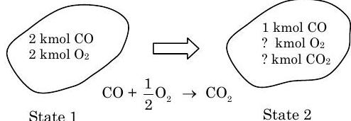
Figure \(\PageIndex{5}\): States 1 and 2 of the system, and the chemical reaction responsible for the change in states.
Analysis:
Strategy \(\rightarrow\) Since this involves mixtures of substances and reactions, use species accounting.
System \(\rightarrow\) Consider a closed system that includes all mass initially in the system.
Property to count \(\rightarrow\) Chemical species
Time period \(\rightarrow\) Since interested in beginning and ending state, use finite-time form.
In general for each species \(j\)
\[\frac{d n_{sys, j}}{d t} = \underbrace{ \cancel{ \sum_{in} \dot{n}_{j, i} - \sum_{out} n_{j, e} }^{=0} }_{\text {closed system}}+\dot{n}_{j, \ gen} - \dot{n}_{j, \ cons} \quad \rightarrow \quad \underbrace{ n_{j, 2} - n_{j, 1} }_{\begin{array}{c} \text{dropped the system} \\ \text{subscript} \end{array}} = n_{j, \ gen} - n_{j, \ cons} \nonumber \]
Now for each species
\[ \begin{align*} & \text{CO:} \quad &\cancel{ n_{\text{CO}, \ 2} }^{=0} + \cancel{ n_{\text{CO}, \ 1} }^{=0} = \cancel{ n_{\text{CO}, \ gen} }^{=0} - n_{\text{CO}, \ cons} \quad &\rightarrow \quad\quad n_{\text{CO}, \ cons} = 1 \ \text{kmol} \\ & \text{O}_2: \quad &n_{\text{O}_2, \ 2} - \cancel{ n_{\text{O}_2, \ 1} }^{=0} = \cancel{ n_{\text{O}_2, \ gen} }^{=0} - n_{\text{O}_2, \ cons} \quad &\rightarrow \quad\quad n_{\text{O}_2, \ 2} = -n_{\text{O}_2, \ cons} \\ &\text{CO}_2: \quad &n_{\text{CO}_2, \ 2} - \cancel{ n_{\text{CO}_2, \ 1} }^{=0} = n_{\text{CO}_2, \ gen} - \cancel{ n_{\text{CO}_2, \ cons} }^{=0} \quad &\rightarrow \quad\quad n_{\text{CO}_2, \ 2} = n_{\text{CO}_2, \ gen} \end{align*} \nonumber \]
This gives us four unknowns and only two equations. To get the remaining equations, look at the chemical reaction equation. In terms of consumption and generation, the chemical reaction is as follows:
\[\begin{gathered} n_{\text {CO}, \ cons} \mathrm{CO} + n_{\text{O}_2, \ cons} \mathrm{O}_2 \rightarrow n_{\text{CO}_2, \ gen} \mathrm{CO}_2 \\[4pt] \mathrm{CO} + \frac{n_{\text{O}_2, \ cons}}{n_{\text {CO}, \ cons}} \mathrm{O}_2 \rightarrow \frac{n_{\text{CO}_2, \ gen }}{n_{\text {CO}, \ cons }} \mathrm{CO}_2 \end{gathered} \nonumber \]
If we compare this equation with the balanced chemical equation for the reaction of \(\mathrm{CO}\) with \(\mathrm{O}_2\) to form \(\mathrm{CO}_2\), we can determine the two remaining equations between the unknowns:
\[\begin{array}{c} \mathrm{CO} + \dfrac{n_{\text{O}_2, cons}}{n_{\text{CO}, \ cons}} \mathrm{O}_2 \rightarrow \dfrac{n_{\text{CO}_2, \ gen}}{n_{\text{CO}, \ cons}} \mathrm{CO}_{2} \\[4pt] \mathrm{CO} + \frac{1}{2} \mathrm{O}_2 \rightarrow \mathrm{CO}_2 \end{array} \quad \Rightarrow \quad \frac{n_{\text{O}_2, \ cons}}{n_{\text{CO}, \ cons}} = \frac{1}{2} \quad \& \quad \frac{n_{\text{CO}_2, \ gen}}{n_{\text{CO}, \ cons}} = 1 \nonumber \]
Thus the final compositions are as follows: \[\begin{align*} &n_{\text{CO}, \ 2} = 1 \ \mathrm{kmol} \\ &n_{\text{O}_2, \ 2} = n_{\text{O}_2, \ gen} = \frac{n_{\text{O}_2, \ gen}}{n_{\text{CO}, \ cons}} n_{\text{CO}, \ cons} = \left( \frac{1}{2} \right) (1 \ \mathrm{kmol}) = \frac{1}{2} \ \mathrm{kmol} \\[4pt] &n_{C\text{O}_2, \ 2} = n_{\text{CO}_2, \ gen} = \frac{n_{\text{CO}_2, \ gen}}{n_{\text{CO}, \ cons}} n_{\text{CO}, cons}=(1)(1 \ \mathrm{kmol}) = 1 \ \mathrm{kmol} \end{align*} \nonumber \]
Comments:
(1) The final mixture has \(3.5 \ \mathrm{kmol}\) compared to \(4.0 \ \mathrm{kmol}\) in the initial mixture. Typically, moles are not conserved.
(2) An alternate approach is to write species accounting equations for the atomic species, \(\text{C}\) and \(\text{O}\). Note that atomic species, like total mass, are conserved.