
5.2: Conservation of Linear Momentum Equation
- Page ID
- 81495

The recommended starting point for any application of the conservation of linear momentum is the rate form of the linear momentum equation (previously given as Equation(5.1.28): \[\frac{d \mathbf{P}_{\text {sys}}}{d t} = \sum \mathbf{F}_{\text {ext}} + \sum_{\text {in}} \dot{m}_{i} \mathbf{V}_{i} - \sum_{\text{out}} \dot{m}_{e} \mathbf{V}_{e} \nonumber \] where \(\mathbf{P}_{\text {sys}}\) is the system linear momentum, \(\mathbf{F}_{\text {ext}}\) is the transport rate of linear momentum by an external force, and \(\dot{m} \mathbf{V}\) is the transport rate of linear momentum by mass flow.
In applying the rate form of the conservation linear momentum to a system, there are many modeling assumptions that are frequently used to build the mathematical model of the physical system. These are detailed in the following paragraphs. As always, you should focus on understanding what the assumptions mean physically and how they can be used to simplify the equations for a given system. Do not just memorize the results.
Steady-state system:
If a system is operating under steady-state conditions, all intensive properties are independent of time, i.e., the values of intensive properties may only vary with position. Thus, the linear momentum of the system is a constant, \(\mathbf{P}_{\text {sys}} = \text{constant}\). When this assumption is applied to the conservation of linear momentum equation, we have
\[\begin{gathered} \cancel{ \underbrace{ \frac{d \mathbf{P}_{\text {sys}}}{d t} }_{ \mathbf{P}_{\text{sys}} = \text{constant} } }^{=0} = \sum \mathbf{F}_{\text {ext}} + \sum_{\text {in}} \dot{m}_{i} \mathbf{V}_{i} - \sum_{\text {out}} \dot{m}_{e} \mathbf{V}_{e} \\ 0 = \sum \mathbf{F}_{\text {ext}} + \sum_{\text {in}} \dot{m}_{i} \mathbf{V}_{i} - \sum_{\text {out}} \dot{m}_{e} \mathbf{V}_{e} \end{gathered} \nonumber \] In words, this says that the net transport rate of linear momentum into the system by force must equal the net transport rate of linear momentum out of the system by mass flow.
Closed system:
A system with boundaries selected so that the mass flow rate at any boundary is identically zero is a closed system; thus the mass of the system is constant. When applied to the conservation of linear momentum, this assumption has the following effect:
\[ \begin{align*} \frac{d \cancel{ \mathbf{P}_{\text{sys}} }^{= m_{\text{sys}} \mathbf{V}_G} }{dt} &= \sum \mathbf{F}_{\text{ext}} + \sum_{\text{in}} \cancel{ \dot{m}_i }^{=0} \mathbf{V}_i - \sum_{\text{out}} \cancel{ \dot{m}_e }^{=0} \mathbf{V}_e \\ m_{\text{sys}} \frac{d \mathbf{V}_G}{dt} + \underbrace{ \cancel{ \frac{d m_{\text{sys}}}{dt} }^{=0} }_{\begin{array}{c} \text{Closed} \\ \text{system} \end{array} } \mathbf{V}_G &= \sum \mathbf{F}_{\text{ext}} \\ m_{\text{sys}} \frac{d \mathbf{V}_G}{dt} &= \sum \mathbf{F}_{\text{ext}} \end{align*} \nonumber \]
where \(\mathbf{V}_{G}\) is the velocity of the center of mass of the system. Recalling that acceleration is just the time derivative of velocity, we immediately recognize that this is our old friend from physics: \(F=m a\).
Closed, steady-state system:
Using what you've learned to this point, how would you expect the linear momentum equation to simplify for a closed system that operates at steady state conditions?
In applying the conservation of linear momentum to model a system, we will need to, as always, select a system and identify the transports of linear momentum across the system boundary. Guidelines for drawing a linear momentum (or free-body) diagram are found below:
- Select a system. Every system can be broken down into smaller subsystems. For a given problem, there may be several possible systems and different questions may require a different system.
- Sketch the physical object clearly identifying the boundaries of your system. This is usually done with a dashed line to indicate the system boundary.
- Detach the system from its surroundings and sketch the isolated contour of the system, i.e., the system boundaries.
- Identify the transports of momentum between the system and the surroundings. When identifying external forces, only consider the forces exerted by the surroundings on the system. Remember that there are two types of external forces: contact (or surface) forces that act on the boundaries of the system and body forces produced by fields like the gravitational force commonly called weight.
- For each momentum transport, draw an arrow on the system diagram showing the direction and location of the transport. Care should be taken to draw each arrow with the correct direction (line-of-action and sense) and position. Label all forces and mass transports of momentum with a name, number, or a symbol. Draw the vector on the diagram by placing either the tail or the head of the arrow at the point of application:
- Contact forces should be applied at the appropriate point on the system boundary where the system was "cut away" from the surroundings.
- The weight vector should be applied at the center of gravity of the body.
- The mass transport of linear momentum vector should be applied at the point where the mass crosses the boundary and in the direction of the velocity.
- If you do not know the correct direction of a momentum transfer, assume a direction. If your analysis results in a negative numerical value for the transfer, then the actual direction is opposite to the direction assumed.
- Draw a coordinate system and indicate all pertinent dimensions and angles on the free-body diagram.
A tennis player serves the ball a distance \(L=40 \ \mathrm{ft}\) back from the net and a height \(H=9 \ \mathrm{ft}\) above the court. The tennis ball leaves the racket with an angle \(\theta=0^{\circ}\) below the horizontal as shown in the figure. The net is \(3 \mathrm{ft}\) high and the center of the tennis ball clears the net by 3 inches. Determine (a) the initial velocity \(V_{o}\) of the ball when it leaves the racket and (b) the distance \(s\) behind the net where the ball hits the court. Assume air drag is negligible. The mass of the tennis ball is \(0.25 \ \mathrm{lbm}\).
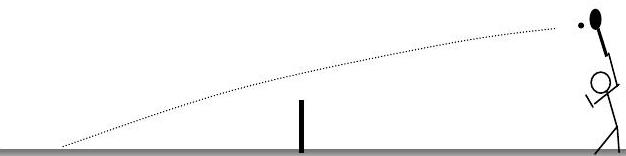
Figure \(\PageIndex{1}\): A tennis player serves a ball.
Solution
Known: Tennis ball is served with a specified angle from a specified location.
Find: (a) The velocity of the ball when it crosses the net and (b) the distance from the net where it hits the court.
Given:
.jpg?revision=1)
Figure \(\PageIndex{2}\): Diagram indicating the path traveled by the ball, assigned a coordinate system and labeled with all relevant measurements.
Analysis:
System \(\rightarrow\) Select the tennis ball as the system. This is a closed system.
Property to count \(\rightarrow\) Since trajectory is governed by effect of gravity, count linear momentum.
Time period \(\rightarrow\) Will eventually need to integrate over finite-time to get trajectory and velocity.
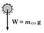
First we must sketch the free-body (linear momentum) diagram for the system. The only transports of linear momentum occur due to the gravity body force-the weight. The inertial coordinate system and the other dimensions are shown on Figure \(\PageIndex{2}\) above.
.jpg?revision=1)
Figure \(\PageIndex{3}\): Free-body diagram of the system.
Writing the rate form of the conservation of linear momentum for the system gives
\[ \frac{ d \mathbf{P}_{\text{sys}}}{dt} = \mathbf{W} + \underbrace{ \cancel{ \left[ \sum_{\text{in}} \dot{m}_i \mathbf{V}_i + \sum_{\text{out}} \dot{m}_e \mathbf{V}_e \right] }^{=0} }_{\text{Closed system, } \dot{m} = 0} \quad \rightarrow \quad \cancel{ \frac{d}{dt} \left( m_{\text{sys }} \mathbf{V}_G \right) }^{=m_{\text{sys}} \frac{d \mathbf{V}_G}{dt}} = m_{\text{sys }} \mathbf{g} \quad \rightarrow \quad m_{\text{sys }} \frac{d \mathbf{V}_G}{dt} = m_{\text{sys }} \mathbf{g} \nonumber \]
Now writing equation in scalar form using the coordinate system defined above and \(\mathbf{V}_G = V_x \mathbf{i} + V_y \mathbf{j}\), we have the following equations:
\[ \cancel{ m_{\text{sys }} } \frac{d \mathbf{V}_G}{dt} = \cancel{ m_{\text{sys }} } \mathbf{g} \quad \rightarrow \quad \frac{d}{dt} \left( V_x \mathbf{i} + V_y \mathbf{j} \right) = -g \mathbf{j} \quad \rightarrow \quad \left\{ \begin{array}{l} x \text {- axis: } \quad \dfrac{d V_{x}}{d t}=0 \\ y \text {-axis: } \quad \dfrac{d V_{y}}{d t}=-g \end{array} \right. \nonumber \]
Integrating once to get velocity gives \[\begin{array}{llllll} x \text {-axis: } & \dfrac{d V_{x}}{d t} = 0 & \rightarrow & V_{x} = \text{constant} = V_{x, o} = V_{o}(\cos \theta) & \rightarrow & V_{x} = V_{o} (\cos \theta) \\ y \text {-axis: } & \dfrac{d V_{y}}{d t} = -g & \rightarrow & \int\limits_{V_{y, o}}^{V_{y}} d V_{y} = -\int\limits_{0}^{t} g \ dt \rightarrow V_{y} - V_{o} (\sin \theta) = -g t & \rightarrow & V_{y} = -g t+V_{o}(\sin \theta) \end{array} \nonumber \]
Now integrating again to get position: \[\begin{array}{lllll} x \text {-axis: } & V_{x} = \dfrac{d x}{d t} = V_{o} \cos \theta & \rightarrow & \int\limits_{0}^{x} d x = \int\limits_{0}^{t} \underbrace{ \left(V_{o} \cos \theta\right) }_{\text{Constant}} \ dt & \rightarrow \quad x = \left(V_{o} \cos \theta\right) t \\ y \text {- axis: } & V_{y} = \frac{d y}{d t} = -gt - V_{o} \sin \theta & \rightarrow & \int\limits_{H}^{y} d x = -\int\limits_{0}^{t} \left(gt+V_{o} \sin \theta\right) \ d t & \rightarrow \quad y-H = -\left(\dfrac{g t^2}{2} + \left(V_{o} \sin \theta \right) t \right) \end{array} \nonumber \]
Now that we know position and velocity as a function of time, let's first solve for the initial velocity required to clear the net at \(x=L\) and \(y=h+d\).
For \(\theta=0\) with \(x\) and \(y\) as specified above, we have two equations for two unknowns \(t\) and \(V_{o}\) : \[\begin{aligned} &x \text {-axis: } \quad\quad\quad\quad\quad\ L = V_{o} t & \rightarrow \quad & \ t =L / V_{o} \\ &y \text {-axis: } \quad (h+d)-H = -\left[\frac{1}{2} g t^{2}\right] & \rightarrow \quad & t^{2} =\frac{2}{g} [H-(h+d)] \end{aligned} \nonumber \]
Combining these equations and eliminating the time \(t\) gives the following result:
\[\begin{gathered} t^{2} = \left( \frac{L}{V_{o}} \right)^{2} = \frac{2}{g}[H-(h+d)] \\ V_{o}^{2} = \frac{g L^{2}}{2[H-(h+d)]} \end{gathered} \quad \rightarrow \quad V_{o} = \sqrt{ \frac{g L^{2}}{2[H-(h+d)]} } = \sqrt{ \frac{ \left(32.2 \ \dfrac{\mathrm{ft}}{\mathrm{s}^{2}} \right)(40 \ \mathrm{ft})^{2}}{2 \left[ 9-\left( 3+\frac{3}{12} \right) \right] \mathrm{ft}}} = 66.9 \ \frac{\mathrm{ft}}{\mathrm{s}} \nonumber \]
Now to solve for \(s\), we recognize that \(s = x - 40\) when \(y=0\) and use the two displacement equations: \[\begin{gathered} s = x-(40 \ \mathrm{ft}) = V_{o} t-(40 \ \mathrm{ft}) \\ 0-H = -\frac{1}{2} g t^{2} \quad \rightarrow \quad H=\frac{1}{2} g t^{2} \end{gathered} \quad \rightarrow \quad s=V_{o} \sqrt{\frac{2 H}{g}-(40 \ \mathrm{ft})} \nonumber \]
Solving for the distance \(s\): \(\quad s = \left( 66.9 \ \dfrac{\mathrm{ft}}{\mathrm{s}}\right) \sqrt{2 \dfrac{(9 \ \mathrm{ft})}{(32.3 \ \mathrm{ft} / \mathrm{s})}} - (40 \ \mathrm{ft}) = 10.0 \ \mathrm{ft}\)
Comments:
- Assuming that the diameter of the tennis ball is 3 inches and the tennis still hits with the initial velocity calculated above, determine the maximum value of \(\theta\) before the ball hits the net.
- Now determine the minimum initial speed that the ball must have to clear the net if it is hit horizontally, e.g. \(\theta=0\).
Water flows steadily through a horizontal nozzle attached to a pipe. The nozzle is flanged and attached to the pipe with 6 bolts as shown in the figure. The pipe and the nozzle inlet has an interior diameter of \(25 \ \mathrm{cm}\) and the outlet diameter of the nozzle is \(12 \ \mathrm{~cm}\). The absolute pressure at the inlet to the nozzle is \(500 \ \mathrm{kPa}\) and the water velocity is \(5 \mathrm{~m} / \mathrm{s}\). The pressure at the nozzle outlet is atmospheric pressure \(\left(P_{\mathrm{atm}}= 100 \mathrm{kPa} \right) \). Assume that the density of liquid water is \(1000 \mathrm{~kg} / \mathrm{m}^{3}\).
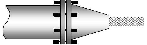
Figure \(\PageIndex{4}\): Water moves through a cylindrical pipe attached to a flanged nozzle.
Determine the total force, in newtons, applied by the bolts to hold the nozzle in place. Assume the bolts only support tension.
Solution
Known: Water flows steadily through a nozzle.
Find: Find the total force exerted by the bolts on the nozzle to hold it in place.
Given:
.jpg?revision=1)
Figure \(\PageIndex{5}\): The pipe and nozzle, assigned with a coordinate system and labeled with all given quantities.
Analysis:
Strategy: Try linear momentum in the \(x\)-direction since the problem asks for forces (a mechanism for transferring linear momentum) and the forces are in the \(x\)-direction.
System \(\rightarrow\) Pick an open, non-deforming system that cuts the pipe at the pipe nozzle connection and includes the nozzle.
Property to count \(\rightarrow\) Try linear momentum and possibly mass (if we need to relate input to output flow rates.
Time period \(\rightarrow\) Looks like it may be a rate (infinitesimal time interval) or steady-state problem.
.jpg?revision=1)
Figure \(\PageIndex{6}\): System choice for this problem.
Starting with the system shown by the dashed line, identify all of the momentum transfers for the system. Walking your fingers around the system boundary you would identify six bolt forces, pressure forces, and the two mass transports of momentum. Now writing these in a vector equation for linear momentum in the \(x\)-direction, we have: \[ \frac{d \mathbf{P}_{x, \text{ sys}}}{dt} = \left[ 6 \mathbf{F}_{\text{bolt, } x} + \mathbf{F}_{\text {net pressure, } x} \right] + \left[ \dot{m} \mathbf{V}_{1, \ x} - \dot{m} \mathbf{V}_{2, \ x} \right] \nonumber \]
A more complete momentum diagram is now required to obtain the correct directions of the forces. The complete diagram is shown below.
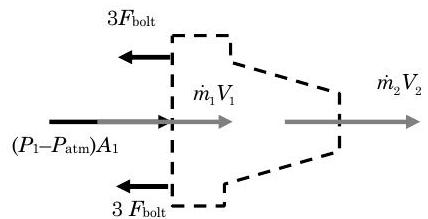.jpg?revision=1)
Figure \(\PageIndex{7}\): Free-body diagram for the nozzle system.
Before continuing, we should explain how we obtained the various terms.
- The mass transport terms are the product of the mass flow rate and the velocity at any flow boundary. The direction of the arrow is in the direction of the velocity.
- Two arrows show the bolt forces. Each arrow represents three (3) bolts. In addition, only the average bolt force can be determined. Note that since the bolts are in tension, the arrows indicate the bolts are pulling on the system.
- The net pressure forces in the \(\mathrm{x}\)-direction must be calculated by considering the pressure distribution over the entire system boundary. As shown in the figure, atmospheric pressure \(P\) atm acts on all surfaces except the inlet flow area where the pressure is \(P_{1}\). Notice that all of the pressure arrows point into the surface. The net force can be determined by subtracting off the atmospheric pressure as shown in the figure. The result is a uniform pressure of \(P_{\text {net }}=P_{1}-P_{\text {atm }}\) acting over the inlet area. The magnitude of the resulting force is \(F_{\text {net pressure, } x} = \left( P_1 - P_{\text {atm}} \right) A_{1}\). This arrow points into the surface and is shown on the momentum diagram above.
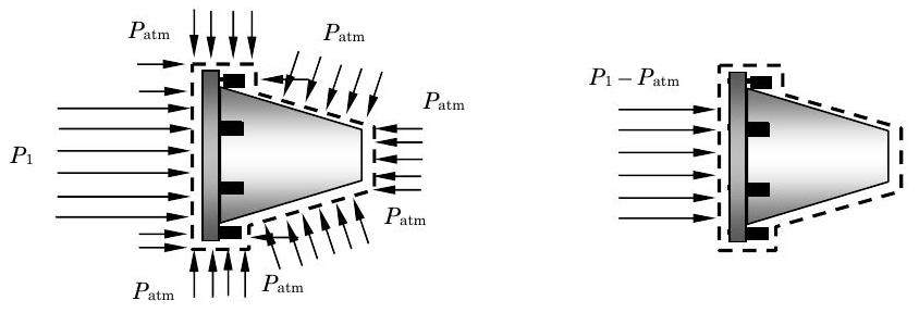
Figure \(\PageIndex{8}\): Equivalent methods of expressing the net pressure experienced by the nozzle system.
Now all that remains is to solve for the bolt forces. Writing the momentum equation as a scalar for the \(\mathrm{x}-\) direction we have:
\[ \begin{align*} & \underbrace{ \cancel{ \frac{d P_{x, \text{ sys}}}{dt} }^{=0} }_{\text{Steady-state}} = \left[ -6 F_{\text{bolt, } x} + \underbrace{ F_{\text{net pressure, } x} }_{= \left( P_1 - P_{\text{atm}} \right) A_1} \right] + \underbrace{ \left[ \dot{m}_1 \left( + V_{1, \ x} \right) - \dot{m}_2 \left( + V_{2, \ x} \right) \right] }_{\begin{array}{c} + \text{ sign for each } V \text{ since a positive value} \\ \text{for } V_{1, \ x} \text{ and } V_{2, \ x} \text{ represents a positive} \\ \text{specific linear momentum} \end{array}} \\[4pt] & 0 = -6 F_{\text{bolt, } x} + \left( P_1 - P_{\text{atm}} \right) A_1 + [ \dot{m}_1 V_1 - \dot{m}_2 V_2 ] \quad \rightarrow \quad 6 F_{\text{bolt, } x} = \left( P_1 - P_{\text{atm}} \right) A_1 + [ \dot{m}_1 V_1 - \dot{m}_2 V_2 ] \end{align*} \nonumber \]
Further simplification can be achieved by applying conservation of mass to the same system and then applying the steady-state assumption:
\[ \cancel{ \frac{d m_{\text{sys}}}{d t} }^{=0} = \dot{m}_1 - \dot{m}_2 \quad \rightarrow \quad \dot{m}_2 = \dot{m}_1 \quad \rightarrow \quad \underbrace{ \cancel{ \rho_1 } A_1 V_1 = \cancel { \rho_2 } A_2 V_2 }_{\text {Incompressible liquid}} \nonumber \]
Using this result, the equation for the bolt forces become \[6 F_{\text {bolt}} = \left( P_{1}-P_{\text {atm}} \right) A_{1} + \dot{m}_{1} \left( V_{1}-V_{2}\right) \nonumber \]
Solving for the area at the inlet: \(A_{1} = \frac{\pi}{4} D_{1}^{2} = \frac{\pi}{4} (0.25 \mathrm{~m})^{2} = 4.909 \times 10^{-2} \mathrm{~m}^{2}\)
Solving for the mass flow rate: \(\dot{m}_{1} = \rho A_{1} V_{1} = \left( 1000 \ \frac{\mathrm{kg}}{\mathrm{m}^{3}} \right) \left( 4.909 \times 10^{-2} \mathrm{~m}^{2} \right) \left( 5 \ \frac{\mathrm{m}}{\mathrm{s}}\right) = 245.5 \ \frac{\mathrm{kg}}{\mathrm{s}}\)
The velocity at the exit becomes: \(V_{2} = \dfrac{A_1}{A_2} V_{1} = \left[ \dfrac{(\pi / 4) D_{1}^{\ 2}}{(\pi / 4) D_{2}^{\ 2}} \right] V_{1} = \left( \dfrac{D_1}{D_2} \right)^{2} V_{1} = \left( \dfrac{25 \mathrm{~cm}}{12 \mathrm{~cm}}\right)^{2} \left( 5 \dfrac{\mathrm{m}}{\mathrm{s}} \right) = 21.70 \ \dfrac{\mathrm{m}}{\mathrm{s}}\)
Substituting these numbers back into the general result gives \[\begin{aligned} 6 F_{\text {bolt}} &= \left( P_{1} - P_{\text {atm}} \right) A_{1} + \dot{m}_{1} \left( V_{1} - V_{2} \right) \\ &=[(500-100) \ \mathrm{kPa}] \left( 4.904 \times 10^{-2} \mathrm{~m}^{2} \right) + \left( 245.5 \ \frac{\mathrm{kg}}{\mathrm{s}} \right) (5.00-21.70) \frac{\mathrm{m}}{\mathrm{s}} \\ &=\left( 19.64 \ \mathrm{kPa} \cdot \mathrm{m}^{2} \right) \left( \frac{1000 \mathrm{~N} / \mathrm{m}^{2}}{\mathrm{kPa}} \right) + \left( -4100 \frac{\mathrm{kg} \cdot \mathrm{m}}{\mathrm{s}^{2}} \right) \left( \frac{\mathrm{N}}{\left( \frac{\mathrm{kg} \cdot \mathrm{m}}{\mathrm{s}^{2}} \right)} \right) \\ &=19.64 \times 10^{3} \mathrm{~N} + \left( -4.10 \times 10^{3} \mathrm{~N} \right) \\ &=15.5 \ \mathrm{kN} \end{aligned} \nonumber \]
Thus the six bolts must exert a total force of \(15.5 \ \mathrm{kN}\) acting to the left (or towards the pipe) to hold the nozzle in place.
Comments:
- Note that the increase in the specific linear momentum, i.e. \(V\), of the mass leaving the system actually serves to reduce the load on the bolts. To see this, consider what the bolt force would be if the nozzle was capped.
- How would the solution change if we had picked the basic \(x\) coordinate to the left instead of to the right as shown? The vector relation would have stayed the same, but the scalar equation would have become as follows
\[ 0 = 6 F_{\text {bolt, }x} - \left(P_{1} - P_{\text {atm}}\right) A_{1} + \left[ \dot{m}_{1} \left( -V_{1} \right) - \dot{m}_{2} \left(-V_{2}\right) \right] \quad \rightarrow \quad 6 F_{\text {bolt, } x} = \left( P_{1} - P_{\text {atm}} \right) A_{1} + \left[ \dot{m}_{1} \left(V_{1}\right) - \dot{m}_{2} \left(V_{2}\right) \right] \nonumber \]
A cable car is pulled along a fixed overhead cable by a cable attached at point \(A\). The car has a mass of \(200 \ \mathrm{kg}\), and the tension in the cable is \(2400 \ \text{N}\). The car is supported by wheels that rest on the cable. The cable is inclined at an angle of \(\theta=22.6^{\circ}\) with the horizontal as shown in the figure.
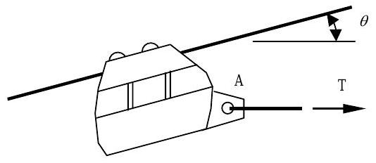
Figure \(\PageIndex{9}\): Cable car suspended from an angled cable is pulled to the right by a horizontal cable.
Determine:
(a) The magnitude and direction of the force \(R\) exerted by the overhead cable on the car wheels, in newtons.
(b) The magnitude and direction of the acceleration of the car in \(\mathrm{m} / \mathrm{s}^{2}\).
Solution
Known: A small inspection car is pulled along a fixed overhead cable by a cable attached at point \(A\)
Find: (a) The magnitude and direction of force \(R\) exerted by the overhead cable on the wheels of the car, in newtons. (b) The magnitude and direction of the acceleration of the car, in \(\mathrm{m} / \mathrm{s}^{2}\).
Given:
\[\begin{aligned} &\mathrm{T} = 2400 \mathrm{~N} \\ & m_{\mathrm{car}}=200 \mathrm{~kg} \\ & \theta = 22.6^{\circ} \end{aligned} \nonumber \]
.jpg?revision=1)
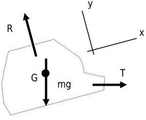
Figure \(\PageIndex{10}\): Free-body diagram of the isolated cable car.
Analysis:
Strategy \(\rightarrow\) Since the problem involves forces, try conservation of linear momentum.
System \(\rightarrow\) Closed system including only the car as shown in the momentum system diagram at right.
Property \(\rightarrow\) Linear Momentum
Time Period \(\rightarrow\) Instantaneous
Without selecting a coordinate system, the conservation of linear momentum equation becomes \[\frac{d}{d t} \mathbf{P}_{\mathrm{sys}}=\sum_{\text {external}} \mathbf{F}_{j} + \sum_{\mathrm{in}} \cancel{ \dot{m}_{i} \mathbf{V}_{i} }^{=0} - \sum_{\text{out}} \cancel{ \dot{m}_{e} \mathbf{V}_{e} }^{=0, \text { closed system}} \quad \rightarrow \quad \frac{d}{d t} \mathbf{P}_{\mathrm{sys}} = m_{\mathrm{sys }} \mathbf{g} + \mathbf{T} + \mathbf{R} \nonumber \] where there are only three external forces - the force on the wheels \(\mathbf{R}\), the weight of the car \(m_{\mathrm{sys }} \mathbf{g}\), and the cable force \(\mathbf{T}\). The net pressure force is zero since atmospheric pressure surrounds the car.
Also, because this is a closed system the linear momentum of the system \(\mathbf{P}_{\text {sys}} = m_{\text {sys}} \mathbf{V}_{G}\) where \(\mathbf{V}_{G}\) is the velocity of the center of mass of the system. Thus, the conservation of linear momentum can now be written as \[\frac{d}{dt} \left( m_{\text{sys }} \mathbf{V}_{\mathrm{G}}\right) = m_{\text{sys }} \mathbf{g} + \mathbf{T} + \mathbf{R} \quad \rightarrow \quad m_{\text{sys }} \frac{d \mathbf{V}_{\mathrm{G}}}{dt} = m_{\text{sys }} \mathbf{g} + \mathbf{T} + \mathbf{R} \nonumber \] Now selecting a coordinate system that is aligned with the cable, the conservation of linear momentum can be written in two components. In the \(y\) direction, the linear momentum equation becomes
\[ m_{\text{sys }} \cancel{ \frac{d V_{G, \ y}}{dt} }^{ \begin{array}{l} =0; \text{ no motion} \\ \text{in } y \text{-direction} \end{array}} = -\left( T \cdot \sin \theta \right) + R - \left( m_{\text{sys }} g \cdot \cos \theta \right) \quad \rightarrow \quad R = \left( T \cdot \sin \theta \right) + \left( m_{\text{sys }} g \cdot \cos \theta \right) \nonumber \]
after solving for the force \(R\).
Substituting in the numerical information gives \[\begin{aligned} R &= (2400 \mathrm{~N}) \cdot \sin \left( 22.6^{\circ} \right) + (200 \mathrm{~kg}) \left(9.81 \ \frac{\mathrm{m}}{\mathrm{s}^{2}}\right) \cdot \cos \left( 22.6^{\circ} \right) \\ &= \quad\quad\quad 922.3 \mathrm{~N} \ \ \quad\quad + \quad\quad\quad 1811 \mathrm{~N} \quad\quad\quad\quad\quad\quad\quad = 2733 \mathrm{~N} \end{aligned} \nonumber \]
In the \(x\) direction, the linear momentum equation becomes \[\begin{aligned} m_{\mathrm{sys}} \frac{d V_{\mathrm{G}, \ x}}{d t} &= (T \cdot \cos \theta) - \left(m_{\text{sys }} g \cdot \sin \theta\right) \\[4pt] \frac{d V_{\mathrm{G}, \ x}}{d t} &= \dfrac{(T \cdot \cos \theta) - \left(m_{\text{sys }} g \cdot \sin \theta\right)}{m_{\mathrm{sys}}}=\left(\frac{T}{m_{\mathrm{sys}}} \cos \theta\right)-(g \cdot \sin \theta) \end{aligned} \nonumber \]
Recalling the definition of acceleration, the \(\mathrm{x}\)-momentum equation can be solved for acceleration as \[a_{\mathrm{G}, \ x} \equiv \frac{d V_{\mathrm{G}, \ x}}{dt} = \left(\frac{T}{m_{\mathrm{sys}}} \cos \theta \right) - (g \cdot \sin \theta) \nonumber \] Substituting in the numerical information gives \[\begin{aligned} a_{\mathrm{G}, \ x} &= \left(\frac{2400 \mathrm{~N}}{200 \mathrm{~kg}}\right) \cos \left(22.6^{\circ}\right) - \left(9.81 \ \frac{\mathrm{m}}{\mathrm{s}^{2}}\right) \sin \left(22.6^{\circ}\right) = \left(12.0 \ \frac{\mathrm{m}}{\mathrm{s}^{2}}\right)(0.9232)-\left(9.81 \ \frac{\mathrm{m}}{\mathrm{s}^{2}}\right)(0.3843) \\[4pt] &=7.31 \ \frac{\mathrm{m}}{\mathrm{s}^{2}} \end{aligned} \nonumber \]
Comments:
- As part of a safety study, determine how the force \(R\) and the car acceleration would change if the pulling cable suddenly broke.
- Following a failure of the pulling cable, the maximum speed of the cable car is limited to \(15 \mathrm{~m} / \mathrm{s}\) by a emergency braking mechanism in the wheel carriage. The braking force is activated when the speed of a "falling" car reaches \(5 \mathrm{~m} / \mathrm{s}\). What braking force must be exerted on the cable car to limit the car speed? If the car is stationary when the pulling cable breaks, how long will it take for the emergency brake to activate and when will the maximum speed be reached?
A scale is used to weigh the water in a tank. Water flows steadily through the tank as shown in the figure. It enters at the top of the tank with volumetric flow rate of \(30 \mathrm{~m}^{3} / \mathrm{s}\) through a pipe with a diameter of \(6 \mathrm{~cm}\). It leaves at the side of the tank through a circular opening with a \(6 \mathrm{-cm}\) diameter. The volume of the water in the tank is \(0.6 \mathrm{~m}^{3}\), and the dry weight of the tank is \(500 \mathrm{~N}\). Determine the scale reading, in newtons.
.png?revision=1)
Figure \(\PageIndex{11}\): Water enters a tank on a scale through Opening 1 and leaves the tank through Opening 2.
Solution
Known: Water flows steadily through a tank that rests on a scale.
Find: The scale reading.
Given:
Inlet Pipe @ 1
Volumetric flow rate \(\dot{V\kern-0.8em\raise0.3ex-}_{1}=30 \mathrm{~m}^{3} / \mathrm{h}\)
Diameter \(D_{1}=6 \mathrm{~cm}\)
Outlet Opening @ 2
Diameter \(D_{2}=6 \mathrm{~cm}\)
Volume of water in tank at steady-state: \(V\kern-1.0em\raise0.3ex-_{\text {water}}=0.6 \mathrm{~m}^{3}\)
Weight of tank: \(W_{\text {tank}}=500 \mathrm{~N}\)
Analysis:
Strategy \(\rightarrow\) Since the problem involves forces, try conservation of linear momentum.
System \(\rightarrow\) Open system that includes all water in the tank and the tank as shown in the momentum system diagram.
Property to count \(\rightarrow\) Linear momentum and mass
Time Period \(\rightarrow\) Instantaneous
.jpg?revision=1)
Figure \(\PageIndex{12}\): Free body diagram of the system consisting of the tank and the water in it.
Writing the rate-form of the conservation of linear momentum equation for this problem gives
\[ \begin{align*} \frac{d \mathbf{P}_{\text {sys}}}{d t} &= \sum_{\text {external}} \mathbf{F}_{j} + \sum_{\text {in}} \dot{m}_{i} \mathbf{V}_{i} - \sum_{\text {out}} \dot{m}_{e} \mathbf{V}_{e} \\ \cancel{ \frac{d \mathbf{P}_{\text{sys}}}{\mathrm{s}} }^{\begin{array}{l} =0 \\ \text {steady state} \end{array}} &= \left(\mathbf{W}_{\text {tank}} + \mathbf{W}_{\text {water}} \right) + \mathbf{F}_{\text {scale}} + \dot{m}_{1} \mathbf{V}_{1} -\dot{m}_{2} \mathbf{V}_{2} \mathrm{~A} \\ 0 &= \left( \mathbf{W}_{\text{tank}} +\mathbf{W}_{\text{water}} \right) + \mathbf{F}_{\text {scale}} +\dot{m}_{1} \mathbf{V}_{1} - \dot{m}_{2} \mathbf{V}_{2} \end{align*} \nonumber \]
Now writing the component of this equation in the y-direction as defined in the figure above, \[0 = \left[ W_{\text {tank}} + W_{\text {water}} \right] -F_{\text {scale}} + \dot{m}_{1} V_{1, y} - \dot{m}_{2} \cancel{ V_{2, y} }^{\begin{array}{l} =0 \\ \text{No } y \text{-component @ 2} \end{array}} \nonumber \]
Solving for \(F_{\text {scale}}\) we have \[F_{\text {scale}} = W_{\text {tank}} + W_{\text {water}} + \dot{m}_{1} V_{1, y} \nonumber \]
Now solving for the weight of the tank \(W_{\text {tank}}\) we have \[W_{\text {water}} = m_{\text {water }} g = \left( \rho_{\text {water}} V_{\text {water}} \right) g = \left(1000 \ \frac{\mathrm{kg}}{\mathrm{m}^{3}} \right) \left( 0.600 \mathrm{~m}^{3} \right) \left( 9.81 \ \frac{\mathrm{m}}{\mathrm{s}^{2}}\right) = 5886 \mathrm{~N} \nonumber \]
The \(\mathrm{y}\)-component of the velocity at 1 and the mass flow rate at 1 are
\[\begin{align*} V_{1, y} = V_{1}=\frac{\dot{V\kern-0.8em\raise0.3ex-}_{1}}{A_{1}} = \frac{\dot{V\kern-0.8em\raise0.3ex-}_{1}}{\left( \dfrac{\pi}{4} D_{1}^{\ 2}\right)} = \frac{\left(30 \ \dfrac{\mathrm{m}^{3}}{\mathrm{h}} \times \dfrac{1 \mathrm{~h}}{3600 \mathrm{~s}} \right)}{\dfrac{\pi}{4} (0.06 \mathrm{~m})^{2}} = 2.95 \ \frac{\mathrm{m}}{\mathrm{s}} \\[4pt] \dot{m}_{1}=\rho_{1} \dot{V\kern-0.8em\raise0.3ex-}_{1} = \left(1000 \ \frac{\mathrm{kg}}{\mathrm{m}^{3}}\right) \left( 30 \ \frac{\mathrm{m}^{3}}{\mathrm{h}} \times \frac{1 \mathrm{~h}}{3600 \mathrm{~s}}\right) = 8.33 \ \frac{\mathrm{kg}}{\mathrm{s}} \end{align*} \nonumber \]
Combining this to solve for the force of the scale on the tank, \(F_{\text {scale}}\): \[\begin{aligned} F_{\text {scale}} &=W_{\text {tank }} + W_{\text {water }} + \dot{m}_{1} V_{1, y} \\ &=(500 \mathrm{~N}) + (5886 \mathrm{~N}) + \left(8.33 \ \frac{\mathrm{kg}}{\mathrm{s}}\right) \left(2.95 \ \frac{\mathrm{m}}{\mathrm{s}}\right) \\ &= (6386 \mathrm{~N}) + (24.6 \mathrm{~N}) \\ &=6411 \mathrm{~N} \end{aligned} \nonumber \]
If the operator had neglected the effect of the water flowing into the tank on the reading, he or she would have overestimated the amount of water in the tank by roughly \(0.4 \%\).
Comment:
What is the magnitude and direction of the horizontal force that the scale must exert on the tank to keep it from sliding off the platform? [Answer: \(24.6 \mathrm{~N} \leftarrow\) ] How could you use a side-force measurement to indicate flow rate?