7.3: Conservation of Energy

The recommended starting point for any application of the conservation of energy is the rate form of the conservation of energy equation:

\[\frac{dE_{\text {sys}}}{dt} = \dot{W}_{\text {net, in}} + \dot{Q}_{\text {net, in}} + \left[\sum_{\text {in}} \dot{m}_{i}\left(h_{i}+\frac{V_{i}^{2}}{2}+g z_{i}\right) - \sum_{\text {out}} \dot{m}_{e}\left(h_{e}+\frac{V_{e}^{2}}{2}+g z_{e}\right)\right] \nonumber \]

Remember, the only restriction built into this equation is that the mass crossing the boundary of the system can only carry with it internal energy, translational kinetic energy, and gravitational potential energy. If a more general form is required, we need only add " \(+e_{\text {other}}\) " after the specific gravitational potential energy term, \(g z\).

In applying this equation to describe the behavior of a system, there are several modeling assumptions that are commonly used. These are described in detail in the following paragraphs. As always, you should focus on understanding the physics underlying the assumption and how they are used. Do not just memorize the simplified equations.

Steady-state system

If a system is operating under steady-state conditions, all intensive properties and interactions are independent of time. Thus, the energy of the system is a constant, \(E_{\text {sys}}= \text{constant}\). When applied to the conservation of energy equation you have

\[\begin{aligned} \underbrace{\cancelto{0}{ \frac{d E_{\text{sys}}}{dt} }}_{E_{\text{sys}} = \text{constant}} &= \dot{W}_{\text {net, in}} + \dot{Q}_{\text {net, in}} + \left[\sum_{\text {in}} \dot{m}_{i} \left(h_{i}+\frac{V_{i}^{2}}{2}+g z_{i}\right) - \sum_{\text {out}} \dot{m}_{e} \left(h_{e}+\frac{V_{e}^{2}}{2}+g z_{e}\right)\right] \\ 0 &= \dot{W}_{\text {net, in}} + \dot{Q}_{\text {net, in}} + \left[\sum_{\text{in}} \dot{m}_{i} \left(h_{i}+\frac{V_{i}^{2}}{2}+g z_{i}\right) - \sum_{\text {out}} \dot{m}_{e} \left(h_{e}+\frac{V_{e}^{2}}{2}+g z_{e}\right)\right] \end{aligned} \nonumber \] In words, the sum of the net transport rates of energy by work, heat transfer, and mass must equal zero.

Closed system

A closed system has no mass flow across its boundary. With this constraint, the conservation of energy equation simplifies as follows: \[\begin{aligned} &\frac{d E_{\text {sys}}}{dt} = \dot{W}_{\text {net, in}} + \dot{Q}_{\text {net, in}} + \underbrace{ \cancelto{0}{ \left[\sum_{\text{in}} \dot{m}_{i} \left(h_{i}+\frac{V_{i}^{2}}{2}+g z_{i}\right) - \sum_{\text {out}} \dot{m}_{e} \left(h_{e}+\frac{V_{e}^{2}}{2}+g z_{e}\right)\right] }}_{\text {No mass flow rates }} \\[4pt] &\frac{d E_{\text {sys}}}{dt} = \dot{W}_{\text {net, in}} + \dot{Q}_{\text {net, in}} \end{aligned} \nonumber \]

Finite-time, closed system

For a closed system over a finite-time interval, you first apply the closed system assumption and then integrate the equation over the specified time interval:

\[\begin{gathered} \frac{d E_{\text {sys}}}{dt} = \dot{W}_{\text{net, in}} + \dot{Q}_{\text{net, in}} + \cancel{ \left[\sum_{\text{in}} \dot{m}_{i} \left(h_{i}+\frac{V_{i}^{2}}{2}+g z_{i}\right) - \sum_{\text{out}} \dot{m}_{e} \left(h_{e}+\frac{V_{e}^{2}}{2}+gz_{e}\right)\right] }^{=0} \\[4pt] \frac{d E_{\text{sys}}}{dt} = \dot{W}_{\text{net, in}} + \dot{Q}_{\text{net, in}} \\ \int\limits_{t_1}^{t_2} \left(\frac{d E_{\text{sys}}}{dt}\right) dt = \int\limits_{t_1}^{t_2} \left(\dot{W}_{\text{net, in}} + \dot{Q}_{\text{net, in}}\right) dt \\ \int\limits_{1}^{2} d E_{\text{sys}} = \int\limits_{1}^{2} \left(\delta W_{\text{net, in}}+\delta Q_{\text{net, in}}\right) \quad \rightarrow \quad \Delta E_{\text{sys}} = W_{\text{net, in}}+Q_{\text{net, in}} \end{gathered} \nonumber \]

In words, this says the change in the energy of the system equals the net transport of energy into the system by work and by heat transfer.

Assumptions about heat transfer and work:

One of the aspects of applying the conservation of energy that frequently puzzles students is the need to say something about the heat transfer and work interactions for the system we are modeling.

Heat transfer:

In this course, we will usually make one of three assumptions about the heat transfer of energy for a system:

1. There is no heat transfer. This is called an adiabatic process or adiabatic system. Physically, applying thermal insulation to the surface approximates an adiabatic surface. Unfortunately, there are no perfect thermal insulators; however, if the time scale of the process is small relative to the time it takes for the heat transfer of energy to occur, then the adiabatic assumption is usually good.
2. The heat transfer \(Q\) or heat transfer rate \(\dot{Q}\) is the unknown we are solving for in the problem.
3. The heat transfer \(Q\) or heat transfer rate \(\dot{Q}\) is given in the problem statement.

Please remember that heat transfer can only be defined with respect to a boundary. If you move the boundary, you change the heat transfer. Without clearly indicating your system boundary, it is impossible to apply any of these assumptions.

The study of heat transfer as a discipline attempts to relate the heat transfer rate at a boundary to other characteristics of the system, such as the thermal conductivity, the convection heat transfer coefficient, and the temperature difference across the boundary. In some problems, you may be given a specific constitutive relation that allows you to calculate the heat transfer rate without using the conservation of energy, similar to our work equations. In all other cases, assume that heat transfer can be modeled using one of the three assumptions listed above.

Work:

In this course we will focus most of our attention on four of the possible work mechanisms. The key to making the correct assumption is to carefully examine the system you select and identify any interactions that look like work. (Physically, imagine walking around the system and looking for any clues that would lead you to believe one of these mechanisms is present.) Remember work is only defined with respect to a boundary. No boundary, no work! Here are some clues for each of the four work mechanisms:

1. Compression-expansion (PdV) work — see if any system boundary is moving in a direction normal to the surface, e.g. a boundary next to a piston.
2. Electric work — see if your system boundary cuts any electrical wires.
3. Shaft work — look to see if your system boundary cuts any rotating shafts.
4. Mechanical work and power — look to see if there are any other forces that move on the boundary of the system.

When we revisit work later we may identify a few more mechanisms; however, this list will suffice for a wide range of important problems.

Assumptions about the substance:: Another new and sometimes puzzling problem students encounter when applying the conservation of energy equation is the need to evaluate thermophysical properties — \(u\), \(h\), \(s\), \(T\), \(P\), \(\rho\), and \(\upsilon\). This requires empirical knowledge about the behavior of the material within the system. This knowledge represents a constitutive equation that allows us to predict the values of the properties once we have identified the state of the substance. We will delay this complication for a while, but shortly we will introduce two substance models that accurately describe the behavior of gases, liquids, and solids under certain conditions.

Example — Motor startup

(adapted from Moran & Shapiro, Thermodynamics)

Under steady-state operating conditions, the shaft of a motor rotates at a constant speed of \(955 \mathrm{~rpm~} (100 \mathrm{~rad} / \mathrm{s})\) and applies a constant torque of \(18 \mathrm{~N} \cdot \mathrm{m}\) to an external load, and the 110-volt motor draws a constant electric current of \(18.2\) amps.

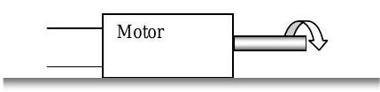
Figure \(\PageIndex{1}\): An electrical motor turns a shaft.

(a) Determine the magnitude and direction of the steady-state heat transfer rate for the motor, in \(\mathrm{kW}\).

(b) During the start-up transient, the rate of heat transfer between the electric motor and its surrounding varies with time as follows: \[\dot{Q}_{\text {out}} = \dot{Q}_{\text {out, ss}} \left[1-e^{-t /(20 \mathrm{~s})}\right] \nonumber \] where \(Q_{\text{out, ss}}\) is the steady-state heat transfer rate from the motor. Obtain an expression for the time rate of change of the energy of the motor using your result from Part (a) and the heat transfer rate equation above.

Solution

Known: A motor operates with known operating conditions

Find: (a) Steady-state heat transfer rate from the motor, in \(\mathrm{kW}\).
(b) Time-rate of change of the motor energy during the startup transient.

Given: During the transient startup: \(\dot{Q}_{\text {out}} = \dot{Q}_{\text {out, ss}} \left[1-e^{-t /(20 \mathrm{~s})}\right]\)

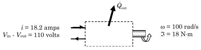
Figure \(\PageIndex{2}\): Known transfers of heat and work between the system of the motor and its surroundings.

Analysis:

Strategy \(\rightarrow\) Because the question involves energy and heat transfer, try the conservation of energy.
System \(\rightarrow\) Take the motor as a closed system
Property to count \(\rightarrow\) Energy
Time period \(\rightarrow\) Both parts appear to require the rate form (infinitesimal time interval)

Sketching a system and identifying the energy transports, we have the figure below.

Figure \(\PageIndex{3}\): System with identified energy transports in and out.

Now applying the closed-system form of the rate form of the conservation of energy equation, we have: \[\frac{d E_{\text {sys}}}{dt} = \dot{W}_{\text {net, in}} + \dot{Q}_{\text {net, in}} = \dot{W}_{\text {electric, in}}-\dot{W}_{\text {shaft, out}}-\dot{Q}_{\text {out}} \nonumber \] where we have used the subscripts to indicate the positive directions corresponding to our diagram

For part (a) we are asked to consider the steady state heat transfer rate, therefore \[\underbrace{ \frac{dE_{\text{sys}}}{dt} }_{\text {Steady state}} = \dot{W}_{\text {electric, in}} - \dot{W}_{\text {shaft, out}} - \dot{Q}_{\text {out}} \quad \rightarrow \quad \dot{Q}_{\text {out}}=\dot{W}_{\text {electric, in}}-\dot{W}_{\text {shaft, out}} \nonumber \]

Now we have to determine the electric power and the shaft power using their defining equations: \[\begin{aligned} \dot{W}_{\text {electric, in }} &= i \cdot \left(V_{\text{in}-\text{o}} - V_{\text{out}-\text{o}}\right) \quad\quad & \dot{W}_{\text{shaft, out}} &= \tau \cdot \omega \\ &=(18.2 \mathrm{~A}) \cdot (110 \mathrm{~V}) & &= (18.0 \mathrm{~N} \cdot \mathrm{m}) \cdot (100 \mathrm{~rad} / \mathrm{s}) \\ &= 2.00 \times 10^{3} \mathrm{~W} & &= 1.80 \times 10^{3} \mathrm{~W} \\ &=2.00 \mathrm{~kW} & &=1.80 \mathrm{~kW} \end{aligned} \nonumber \]

Substituting these results back into the steady-state energy balance, we have \[\dot{Q}_{\text {out}}=\dot{W}_{\text {electric, in}}-\dot{W}_{\text {shaft, out}} = (2.00-1.80) \mathrm{~kW}=0.20 \mathrm{~kW} \nonumber \]

Now for part (b), we are interested in rate of energy storage in the motor, not the amount of energy stored in the motor. Starting with the rate form of the energy balance we have \[\frac{d E_{\text{sys}}}{dt} = \dot{W}_{\text {electric, in}}-\dot{W}_{\text {shaft, out}}-\dot{Q}_{\text {out}} = \dot{W}_{\text {electric, in}}-\dot{W}_{\text {shaft, out}} - \dot{Q}_{\text {out, ss}} \left[1-e^{-t /(20 \mathrm{~s})}\right] \nonumber \] after substituting in the given information for the heat transfer rate.

Assuming that the shaft and electric powers are constant during this transient will give the following result: \[\begin{aligned} \frac{d E_{\text{sys}}}{dt} &= \dot{W}_{\text {electric, in}}-\dot{W}_{\text {shaft, out}}-\dot{Q}_{\text {out, ss}} \left[1-e^{-t /(20 \mathrm{~s})}\right] \\ &= (2.00 \mathrm{~kW})-(1.800 \mathrm{~kW})-(0.20 \mathrm{~kW}) \left[1-e^{-t /(20 \mathrm{~s})}\right] = (0.20 \mathrm{~kW}) e^{-t /(20 \mathrm{~s})} \end{aligned} \nonumber \] Thus the time rate of change is greatest at \(t=0\) and then decreases exponentially.

Comments:

(1) The assumption that the electric power and the shaft power are constant during this startup transient is probably incorrect. A more accurate model of the motor would require a motor performance curve that shows torque and electric current as a function of rotational speed. Typically, when a motor starts up the current surges to provide the necessary startup torque. A portion of the system energy would be stored in the rotational kinetic energy of the rotor as it spins up.

(2) How does the energy inside the system as a function of time? To do this you must integrate the rate of change with time. What's the maximum change? Is there one? Try it and see what you get. Answer: \(\Delta E=(4.0 \mathrm{~kJ}) \left[1-e^{-t /(20 \mathrm{~s})}\right]\)

Example — Refrigerant Compressor

A refrigeration system includes a compressor that takes in refrigerant at State 1 and discharges the refrigerant at State 2. Available state information is shown in the figure. The power input to the compressor is \(2.2 \mathrm{~kW}\). The mass flow rate of refrigerant is \(0.014 \mathrm{~kg} / \mathrm{s}\).

Determine (a) the direction and magnitude of the heat transfer rate and (b) the shaft torque if the compressor power is supplied as shaft work and the compressor operates at \(600 \mathrm{rpm}\).

Figure \(\PageIndex{4}\): System of refrigerant compressor, with all known information about the refrigerant's entering and exiting states.

Solution

Known: A compressor operates at steady-state conditions.

Find: Determine the steady-state heat transfer rate and shaft torque for the compressor.

Given: State, power, and shaft information as included in the problem statement above. [Students, this information is not repeated here because it is so clearly stated above; however, if you were preparing an engineering solution for the record, you should use this space to document all of the information and symbols gleaned from the problem.]

Analysis:

Strategy \(\rightarrow\) Again, since we are talking about energy, try the conservation of energy and mass.
System \(\rightarrow\) Treat the compressor as a non-deforming open system with one inlet and one outlet
Property \(\rightarrow\) Energy and mass (since it is an open system)
Time interval \(\rightarrow\) Infinitesimal time interval, rate form

Starting with a system diagram shown below, we have a heat transfer rate in, a shaft power in, and two places where mass crosses the boundary of the system.

Figure \(\PageIndex{5}\): Mass and energy transfers into/out of the compressor system.

Writing the rate form of the energy balance and the mass balance for this system we have the following:

\[ \begin{aligned} & \text{Energy:} \quad\quad \underbrace{ \cancel{\frac{d E_{\text{sys}}}{dt}}^{=0} }_{\text {Steady state}} = \dot{W}_{\text {shaft, in}}+\dot{Q}_{\text {in}} + \dot{m}_{1}\left(h_{1}+\frac{V_{1}{ }^{2}}{2}+g z_{1}\right) - \dot{m}_{2}\left(h_{2}+\frac{V_{2}{ }^{2}}{2}+g z_{2}\right) \\ & \text{Mass:} \quad\quad \underbrace{ \cancel{\frac{d m_{\text {sys}}}{dt}}^{=0} }_{\text {Steady state}} = \dot{m}_{1}-\dot{m}_{2} \quad \rightarrow \quad \dot{m}_{1}=\dot{m}_{2}=\dot{m} \end{aligned} \nonumber \]

Combining these results and solving for the heat transfer rate we have the following:

\[ \begin{gathered} 0 = \dot{W}_{\text{shaft, in}} + \dot{Q}_{\text{in}} + \dot{m}_{\text{in}} \left[ \left(h_{1}-h_{2}\right) + \left(\frac{V_{1}{ }^{2}}{2} - \frac{V_{2}{ }^{2}}{2}\right) + \underbrace{ g \cancel{ \left(z_{1}-z_{2}\right) }^{=0} }_{\begin{array}{c} \text{No information about} \\ \text{change in elevation given.} \\ \text{Assume this is negligible.} \end{array}} \right] \\ \dot{Q}_{\text{in}} = - \dot{W}_{\text{shaft, in}} - \dot{m}_{\text{in}} \left[\left(h_{1}-h_{2}\right) + \left(\frac{V_{1}{ }^{2}}{2} - \frac{V_{2}{ }^{2}}{2}\right) \right] \end{gathered} \nonumber \]

where we have explicitly recognized that we know nothing about the change in elevation and thus have assumed it will be insignificant. (We have not forgotten it. We have consciously made a modeling assumption.)

(a) Now to solve for the heat transfer we must substitute information back into the energy balance:

\[\begin{aligned} \dot{Q}_{\text{in}} &= -(2.2 \mathrm{~kW}) - \left(0.014 \frac{\mathrm{~kg}}{\mathrm{s}}\right) \left[(1449.8-1590.3) \ \frac{\mathrm{kJ}}{\mathrm{kg}} + \left(\frac{50^{2}-105^{2}}{2}\right) \left(\frac{\mathrm{m}}{\mathrm{s}}\right)^{2}\right] \\ &= -(2.2 \mathrm{~kW}) - \left(0.014 \ \frac{\mathrm{kg}}{\mathrm{s}}\right) \left[(-140.5) \ \frac{\mathrm{kJ}}{\mathrm{kg}} + (-4262.5) \frac{\mathrm{m}^{2}}{\mathrm{~s}^{2}} \times \left(\frac{1 \mathrm{~kJ}}{1000 \mathrm{~N} \cdot \mathrm{m}}\right) \times \left(\frac{1 \mathrm{~N}}{ \dfrac{\mathrm{~kg} \cdot \mathrm{m}}{\mathrm{s}^{2}} }\right)\right] \\ &= -(2.2 \mathrm{~kW})-\underbrace{\left(0.014 \ \frac{\mathrm{kg}}{\mathrm{s}}\right) \left[(-140.5) \ \frac{\mathrm{kJ}}{\mathrm{kg}} + (-4.2625) \ \frac{\mathrm{kJ}}{\mathrm{kg}}\right]}_{-2.027 \mathrm{~kW}} \\ &= -0.173 \mathrm{~kW} \end{aligned} \nonumber \]

Thus the heat transfer rate for the compressor is \(0.173 \mathrm{~kW}\) out of the system. Typically, you might say "the compressor loses energy by heat transfer at the rate of \(0.173 \mathrm{~kW}\)."

(b) Now to find the shaft torque we have to look at the shaft power and apply the definition of shaft power: \[\begin{aligned} \dot{W}_{\text {shaft, in}} = \tau \cdot \omega \quad \rightarrow \quad \tau &= \frac{\dot{W}_{\text {shaft, in}}}{\omega} = \frac{2.2 \mathrm{~kW}}{600 \mathrm{~rpm}} \times \frac{\left(\frac{1 \mathrm{~kN} \cdot \mathrm{m}}{\mathrm{s} \cdot \mathrm{kJ}}\right)}{\left(\dfrac{\mathrm{rev} / \mathrm{min}}{\mathrm{rpm}}\right) \times \left(\dfrac{2 \pi \mathrm{~rad}}{\mathrm{rev}}\right)} \\ &= \frac{\left(2.2 \ \dfrac{\mathrm{kN} \cdot \mathrm{m}}{\mathrm{s}}\right)}{\left(1200 \pi \ \dfrac{\mathrm{rad}}{\mathrm{min}}\right)} \times \left(\frac{60 \mathrm{~s}}{\mathrm{~min}}\right) = 0.0350 \mathrm{~kN} \cdot \mathrm{m} = 35.0 \mathrm{~N} \cdot \mathrm{m} \end{aligned} \nonumber \] The shaft torque applied to the compressor will have the same sense as the direction of shaft rotation.

Comment

(1) Notice how we have explicitly indicated our assumptions as we moved from the most general form of the conservation equations to the specific form of the equation used to model this system.

(2) Typically, the only properties at state 1 and 2 that we could have measured would be \(P\), \(T\), and \(V\). All of the other properties would have been found from tables or equations that relate \(u\), \(h\), and \(\upsilon\) to \(P\) and \(T\).

Example — Steam separator

Most steam power plants have a device that separates steam (gaseous water) from liquid water before it enters the steam turbine. The figure below shows one example. Experience has shown that droplets of liquid water, even small ones, can significantly erode the blades in a steam turbine.

A mixture of liquid water and steam enters a separator vessel at 1 with a mass flow rate of \(10,000 \mathrm{~lbm} / \mathrm{h}\). Steam exits the vessel at 2 and liquid water exits the vessel at 3. The separator operates adiabatically at steady-state conditions with negligible changes in kinetic and gravitational potential energy. Measurements on the vessel indicate that when the system is operating at \(2000 \mathrm{~psia}\), the specific enthalpies and specific volumes of the three streams are as follows: \[\begin{array}{lll} h_{1}=787.7 \mathrm{~Btu} / \mathrm{lbm}; & h_{2}=1136.1 \mathrm{~Btu} / \mathrm{lbm}; & h_{3}=671.6 \mathrm{~Btu} / \mathrm{lbm}; \\ \mathrm{\upsilon}_{1}=0.0662 \mathrm{~ft}^{3} / \mathrm{lbm}; & \mathrm{v}_{2}=0.1881 \mathrm{~ft}^{3} / \mathrm{lbm}; & \mathrm{v}_{3}=0.02563 \mathrm{~ft}^{3} / \mathrm{lbm} \end{array} \nonumber \]

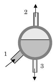
Figure \(\PageIndex{6}\): Steam separator with three openings.

Determine (a) the mass flow rates at 2 and 3, and (b) the flow areas at 1 and 3 assuming the velocity is \(15 \mathrm{~ft} / \mathrm{s}\).

Solution

Known: A steam separator operates at adiabatic, steady-state conditions.

Find: (a) Mass flow rates leaving the vessel
(b) Fluid velocities at all flow cross-sections assuming a \(15 \mathrm{~ft} / \mathrm{s}\) velocity.

Given: See figure above.

Analysis:

Strategy \(\rightarrow\) Try conservation of mass.
System \(\rightarrow\) Take the vessel as a non-deforming open system.
Property to count \(\rightarrow\) Mass
Time interval \(\rightarrow\) Infinitesimal interval, rate form

Figure \(\PageIndex{7}\): System boundary and the mass flows across it.

Sketching the system diagram, we have three mass flows crossing the system boundary as shown in the sketch. Now writing the equations for conservation of mass, we have the following:

\[\text {Mass:} \quad\quad \underbrace{ \cancel{\frac{dm_{\text{sys}}}{dt}}^{=0} }_{\text {Steady-state}} = \dot{m}_{1}-\dot{m}_{2}-\dot{m}_{3} \quad \rightarrow \quad \dot{m}_{3}=\dot{m}_{1}-\dot{m}_{2} \nonumber \]

Unfortunately there are two unknowns, so we need another equation. (Notice that our strategy is being revised as we work, since we didn't notice that conservation of mass would give us one equation with two unknowns.) To get another equation, apply the conservation of energy to this system: \[ \text{Energy:} \quad\quad \underbrace{ \cancel{\frac{d E_{\text{sys}}}{d t}}^{=0} }_{\text {Steady state}} = \underbrace{ \cancel{ \dot{Q}_{\text {net, in}} }^{=0}}_{\text {Adiabatic}} + \underbrace{ \cancel{ \dot{W}_{\text {net, in}} }^{=0}}_{\begin{array}{c}\text {Nothing on boundary} \\ \text {looks like power}\end{array}} + \underbrace{\dot{m}_{1} h_{1}-\dot{m}_{2} h_{2}-\dot{m}_{3} h_{3}}_{\begin{array}{c} \text {Neglecting kinetic and potential} \\ \text {energy per the problem statement}\end{array}} \quad \rightarrow \quad 0=\dot{m}_{1} h_{1}-\dot{m}_{2} h_{2}-\dot{m}_{3} h_{3} \nonumber \]

The energy equation has the same two unknowns — the mass flow rates at 2 and 3. Substituting in the values from the problem statement and solving simultaneously gives the following: \[\left. \begin{array}{l} \dot{m}_{3}=\left(10000 \ \dfrac{\mathrm{lbm}}{\mathrm{h}}\right)-\dot{m}_{2} \\ 0=\left(10000 \ \dfrac{\mathrm{lbm}}{\mathrm{h}}\right) \left(778.7 \ \dfrac{\mathrm{Btu}}{\mathrm{lbm}}\right) - \dot{m}_{2}\left(1136.1 \ \dfrac{\mathrm{Btu}}{\mathrm{lbm}}\right) - \dot{m}_{3}\left(671.6 \ \dfrac{\mathrm{Btu}}{\mathrm{lbm}}\right) \end{array} \right\} \quad \rightarrow \quad \left\{ \begin{array}{l} \dot{m}_{2}=2.50 \times 10^{3} \mathrm{~lbm} / \mathrm{h} \\ \dot{m}_{3}=7.50 \times 10^{3} \mathrm{~lbm} / \mathrm{h} \end{array}\right. \nonumber \] So roughly \(25 \%\) of the entering water leaves the vessel as steam and \(75 \%\) leaves the vessel as liquid water.

Now to find the cross-sectional areas if the velocity is \(15 \mathrm{~ft} / \mathrm{s}\), we can make use of the definition of mass flow rate as follows: \[\begin{aligned} &\dot{m}=\rho V A_{c} = \frac{V A_{c}}{\upsilon} \rightarrow A_{c}=\frac{\dot{m} \upsilon}{V} = \frac{\dot{m} \upsilon}{\left(15 \ \dfrac{\mathrm{ft}}{\mathrm{s}} \times \dfrac{3600 \mathrm{~s}}{\mathrm{~h}}\right)} = \frac{\dot{m} \upsilon}{\left(54000 \ \dfrac{\mathrm{ft}}{\mathrm{h}}\right)} \\ & \text {At 1:} \quad A_{c, \ 1} = \frac{\left(10,000 \ \dfrac{\mathrm{lbm}}{\mathrm{h}}\right) \left(0.0662 \ \dfrac{\mathrm{ft}^{3}}{\mathrm{lbm}}\right)}{\left(54000 \ \dfrac{\mathrm{ft}}{\mathrm{h}}\right)} = 12.3 \times 10^{-3} \ \mathrm{ft}^{2}=1.77 \ \mathrm{in}^{2} \\ & \text {At 3:} \quad A_{c, \ 3} = \frac{\left(7500 \ \dfrac{\mathrm{lbm}}{\mathrm{h}}\right) \left(0.02563 \ \dfrac{\mathrm{ft}^{3}}{\mathrm{lbm}}\right)}{\left(54000 \ \dfrac{\mathrm{ft}}{\mathrm{h}}\right)} = 3.56 \times 10^{-3} \ \mathrm{ft}^{2}=0.513 \ \mathrm{in}^{2} \end{aligned} \nonumber \] Notice how the area at \(3\) is approximately \(30 \%\) of the area at \(1\), even though the mass flow rate is only \(77 \%\) of the mass flow rate at \(1\). This is the result of the changes in fluid specific volume.

Comments

(1) Notice how in this problem we were forced to use both the energy and the mass balances to get sufficient equations for solving the problem. Often our initial strategy will be incorrect. A hallmark of a good problem solved is the ability to not get locked into a single approach. Be flexible.

(2) If the entering mass flow rate had not been given, we could still have solved for the mass flow split in the separator. To do this, we divide both the mass and energy equations through by one of the three unknown flow rates, say the mass flow rate at 1 : \[\begin{array}{c} 0 = \dot{m}_{1}-\dot{m}_{2}-\dot{m}_{3} \\ 0=\dot{m}_{1} h_{1}-\dot{m}_{2} h_{2}-\dot{m}_{3} h_{3} \end{array} \quad \rightarrow \quad \begin{array}{c} 0=1-\dfrac{\dot{m}_{2}}{\dot{m}_{1}}-\dfrac{\dot{m}_{3}}{\dot{m}_{1}} \\ 0=h_{1} - \left(\dfrac{\dot{m}_{2}}{\dot{m}_{1}}\right) h_{2}-\left(\dfrac{\dot{m}_{3}}{\dot{m}_{1}}\right) h_{3} \end{array} \nonumber \] In this way, we've gone from three unknowns to two unknowns and now have sufficient equations to solve for the split. Open system problems are often solved on a "per unit mass" basis by dividing everything in the equation by a mass flow rate and eliminating one unknown.

Example — Making the rounds

A gas is contained inside of a simple piston cylinder device and initially occupies a volume of \(0.020 \mathrm{~m}\) and at a pressure of \(1.0 \mathrm{~MPa}\). The gas executes three processes in series and returns to its initial state as described below:

State 1: \(P_{1}=1.0 \mathrm{~MPa}, V\kern-0.8em\raise0.3ex-_{1}=0.020 \mathrm{~m}^{3}\)

Process 1 \(\rightarrow\) 2: Polytropic expansion with \(P V\kern-1.0em\raise0.3ex-^{1.4}=C\)

State 2: \(V\kern-1.0em\raise0.3ex-_{2} = 2 V\kern-0.8em\raise0.3ex-_{1}\)

Process 2 \(\rightarrow\) 3: Constant volume heating

State 3: \(P_{3}=P_{1}, \quad V\kern-1.0em\raise0.3ex-_{3} = V\kern-0.8em\raise0.3ex-_{2}\)

Process 3: \(\rightarrow\) 1: Constant pressure compression

(This is called a thermodynamic cycle because the system executes a series of processes and then returns to its initial state.) Assume that changes in kinetic and gravitational potential energy are negligible for all processes.

Figure \(\PageIndex{8}\): System consisting of the gas inside a cylinder piston device.

Determine (a) the work done on the gas inside the piston for each process; (b) the net work for the entire cycle, i.e. sum of the work for each process in the cycle; (c) the heat transfer for the entire cycle.

Solution

Known: A gas contained in a piston-cylinder device executes a three-process cycle.

Find: (a) work done on the gas for each process
(b) net work done on the gas for the cycle.
(c) net heat transfer for the entire cycle.

Given: See figure and state/process information above.

Analysis:

Strategy \(\rightarrow\) Should require the use of conservation of energy and may be able to use the definition of \(\mathrm{PdV}\) work to evaluate the work for at least some of the processes.
System \(\rightarrow\) Closed, deforming system consisting of the gas in the cylinder (see dashed line)
Property to count \(\rightarrow\) Energy
Time interval \(\rightarrow\) Should be finite time since each process has a definite beginning and ending.

(a) The only type of work that is possible for this system is compression-expansion \((\mathrm{PdV})\) work. Assuming that each process occurs slow enough so that the pressure is uniform inside the gas throughout the process we have the following equation: \[W_{\text{PdV, in}} = -\int\limits_{1}^{2} P \ d V\kern-0.8em\raise0.3ex- \nonumber \] The trick then is to evaluate it for each process as required.

Process \(1 \rightarrow 2\) : Polytropic process with \(P V\kern-1.0em\raise0.3ex-^{1.4} =C\). Integrating subject to this constraint, we have

\[ \begin{aligned} W_{1-2, \text{ in}} &= - \int\limits_{1}^{2} P \ d V\kern-1.0em\raise0.3ex- = - \int\limits_{V\kern-0.5em\raise0.3ex-_{1}}^{V\kern-0.5em\raise0.3ex-_{2}} \frac{C}{V\kern-0.8em\raise0.3ex-^{1.4}} \ d V\kern-1.0em\raise0.3ex- = -C \int\limits_{V\kern-0.5em\raise0.3ex-_{1}}^{V\kern-0.5em\raise0.3ex-_{2}} V\kern-1.0em\raise0.3ex-^{1.4} \ d V\kern-1.0em\raise0.3ex- = -C\left[ \frac{1}{-1.4+1} V\kern-1.0em\raise0.3ex-^{(-1.4+1)}\right]_{V\kern-0.5em\raise0.3ex-_{1}}^{V\kern-0.5em\raise0.3ex-_{2}} = \frac{C}{1.4-1} \left[V\kern-1.0em\raise0.3ex-_{2}{ }^{-0.4} - V\kern-1.0em\raise0.3ex-_{1}{ }^{-0.4}\right] \\ &= \frac{\left(P_{1} V\kern-1.0em\raise0.3ex-_{1}{ }^{1.4}\right)}{0.4} \left(V\kern-1.0em\raise0.3ex-_{1}{ }^{-0.4}\right) \left[ \left(\frac{V\kern-0.8em\raise0.3ex-_{2}}{V\kern-0.8em\raise0.3ex-_{1}}\right)^{-0.4} - 1\right] = 2.5 \left(P_{1} V\kern-1.0em\raise0.3ex-_{1}\right) \left[ \left(\frac{V\kern-0.8em\raise0.3ex-_{2}}{V\kern-0.8em\raise0.3ex-_{1}}\right)^{-0.4} - 1\right] \\ &= 2.5 \left[\left(1000 \mathrm{~kPa}\right) \left(0.020 \mathrm{~m}^{3}\right)\right] \left[\left(\frac{2}{1}\right)^{-0.4} - 1\right] = \left(-12.1 \mathrm{~kPa} \cdot \mathrm{m}^{3}\right) \times \left( \frac{\mathrm{N} / \mathrm{m}^{3}}{\mathrm{Pa}} \right) = -12.1 \mathrm{~kN} \cdot \mathrm{m} \end{aligned} \nonumber \]

Process 2 \(\rightarrow\) 3 : Constant volume heating

Since there is no volume change and \(\mathrm{PdV}\) work is the only kind possible here, \(W_{2-3, \text { in}}=0\).

Process 3 \(\rightarrow\) 1: Constant pressure cooling \[W_{3-1, \text { in}} = -\int\limits_{3}^{1} P \ d V\kern-0.8em\raise0.3ex- = -P_{3} \left(V\kern-1.0em\raise0.3ex-_{1} - V\kern-0.8em\raise0.3ex-_{3}\right) = -P_{3} \left(V\kern-1.0em\raise0.3ex-_{1} - V\kern-0.8em\raise0.3ex-_{2}\right) \quad \text { because } V\kern-0.8em\raise0.3ex-_{3} = V\kern-0.8em\raise0.3ex-_{2} \nonumber \]

But we already know that for State 2 \(V\kern-0.8em\raise0.3ex-_{2} = 2 V\kern-0.8em\raise0.3ex-_{1}\). Combining this give us the work for process 3 \(\rightarrow\) 1: \[W_{3-1, \text { in}} = -P_{3} \left(V\kern-1.0em\raise0.3ex-_{1} - V\kern-0.8em\raise0.3ex-_{2}\right) = -(1000 \mathrm{~kPa})(0.020-0.040) \mathrm{~m}^{3} = 20.0 \mathrm{~kN} \cdot \mathrm{m} \nonumber \]

(b) To find the net work for the cycle we just add up the three work terms: \[W_{\text {cycle, net in}} = W_{1-2, \text { in}} + W_{2-3, \text { in}} + W_{3-1, \text { in}} = [(-12.1)+0+20.0] \mathrm{~kN} \cdot \mathrm{m} = 7.9 \mathrm{~kN} \cdot \mathrm{m} = 7.9 \mathrm{~kJ} \nonumber \]

(c) To find the net heat transfer of energy, we will resort to the finite-time energy balance for a closed system \[\begin{array}{l} \quad\,\,\ \text{ Process } 1 \rightarrow 2: \quad \Delta E = E_{2}-E_{1} = Q_{1-2, \text { in}}+W_{1-2, \text { in}} \\ \quad\,\,\ \text{ Process } 2 \rightarrow 3: \quad \Delta E = E_{3}-E_{2} = Q_{2-3, \text { in}}+W_{2-3, \text { in}} \\ \underline{ +\quad \text {Process } 3 \rightarrow 1: \quad \Delta E = E_{1}-E_{3} = Q_{3-1, \text{ in}}+W_{3-1, \text{ in}} } \\ \underbrace{\left(E_{2}-E_{1}\right) + \left(E_{3}-E_{2}\right) + \left(E_{1}-E_{3}\right)}_{=0} = \underbrace{\left(Q_{1-2, \text { in}} + Q_{2-3, \text { in}} + Q_{3-1, \text { in}}\right)}_{Q_{\text {cycle, net in}}} + \underbrace{\left(W_{1-2, \text { in}}+W_{2-3, \text { in}}+W_{3-1, \text { in}}\right)}_{W_{\text {cycle, net in}}} \end{array} \nonumber \]

Thus we have \(0=Q_{\text {cycle, net in}} + W_{\text {cycle, net in}}\)

And for the net heat transfer rate for the cycle we have \(Q_{\text {cycle, net in}} = -W_{\text {cycle, net in}}=7.9 \mathrm{~kJ}\)

Comment

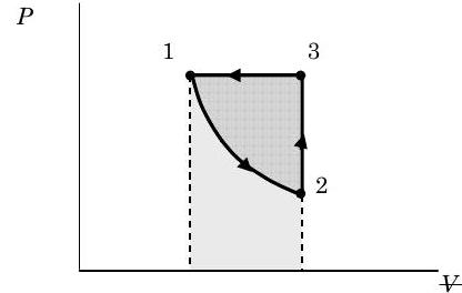
The figure below shows the various areas that correspond to the work for the various processes. The rectangle under line 3-1 represents the work for Process 3 \(\rightarrow\) 1 and the area under the curve 1-2 represents the work for Process 1 \(\rightarrow\) 2. The area enclosed inside the closed curve 1-2-3 represents the net work for the cycle. If we had reversed the direction of the cycle, how would the values of \(Q\) and \(W\) change for the cycle?

Figure \(\PageIndex{9}\): Graph of pressure against volume for the gas as it undergoes the three processes.

Example — They say there's resistance

A 12-volt auto battery is connected to a \(100 \text{ k} \Omega \ (100 \text{ kilo-ohm})\) resistor. Assume changes in kinetic and gravitational potential energy are negligible and that the battery voltage and current do not change with time for the period of this problem. Measurements indicate that the heat transfer rate from the battery is approximately \(2 \%\) of the electric power it delivers.

Figure \(\PageIndex{10}\): Battery connected to a 100 kilo-Ohm resistor.

Determine: (a) the rate of change of the internal energy of the battery, in \(\mathrm{J} / \mathrm{s}\); (b) the heat transfer rate for the resistor, in watts.

Solution

Known: A 12 -volt car battery is connected to a \(100-\mathrm{k} \Omega\) resistor

Find: (a) Rate of change of internal energy of the battery, in \(\mathrm{kJ} / \mathrm{s}\).
(b) Heat transfer rate for the resistor, in \(\mathrm{kW}\).

For the battery:

\(\dot{Q}_{\text {battery, out}}=(0.02) \cdot \dot{W}_{\text {battery, out}}\)

\(V^{+}-V^{-}=12 \text{ volts}\)

For the resistor: \(R=100 \mathrm{~k} \Omega\)

Figure \(\PageIndex{11}\): Separating the circuit into systems for analysis.

Analysis:

Strategy \(\rightarrow\) Because we are interested in internal energy changes and heat transfer, try conservation of energy.
System \(\rightarrow\) May need to use both battery and resistor.
Property to count \(\rightarrow\) Energy.
Time interval \(\rightarrow\) Infinitesimal time interval, rate form of equations.

Before we can solve for any other information, we will need to know the electric current flowing in the system. Assuming that the resistor obeys Ohm's Law, then \[\Delta V = i R \quad \rightarrow \quad i=\frac{\Delta V}{R} = \frac{(12 \mathrm{~V})}{\left(100 \times 10^{3} \ \Omega\right)} \times \left(\frac{1 \mathrm{~A} \cdot \Omega}{\mathrm{V}}\right) = 12 \times 10^{-5} \mathrm{~A}=0.12 \mathrm{~mA} \nonumber \]

Now to answer part (a), let's consider a system that includes the battery and some of the wires as shown above. Applying the energy balance to this closed system we have \[\underbrace{ \cancel{\frac{d E_{\text{sys}}}{dt}}^{=U} }_{\begin{array}{c} \text {Neglecting all} \\ \text {but internal energy} \end{array}} = -\dot{W}_{\text{out}} - \cancel{ \dot{Q}_{\text{out}} }^{=0.02 \dot{W}_{\text {out}}} \quad \rightarrow \quad \frac{d U_{\text{battery}}}{dt} = -\dot{W}_{\text {out}} - 0.02 \dot{W}_{\text {out}} = -1.02 \cdot \dot{W}_{\text {out}} \nonumber \]

To continue requires using our definition for electric power as follows: \[\begin{aligned} \frac{d U_{\text {battery}}}{d t} &= (-1.02) \cdot \dot{W}_{\text {electric, out}} = (-1.02) \cdot(i \Delta V) \\ &=(-1.02) \cdot[(0.12 \mathrm{~mA}) \cdot (12 \text { volts})] = (-1.02) \cdot \underbrace{\left[1.44 \times 10^{-3} \mathrm{~W}\right]}_{\dot{W}_{\text {battery, out}}} = -1.47 \times 10^{-3} \ \frac{\mathrm{J}}{\mathrm{s}} \end{aligned} \nonumber \]

Notice that even though the battery has a constant voltage difference and a constant current, it is not a steady-state system. This should make physical sense as the battery is supplying energy to another system; thus, its internal energy should be decreasing.

For part (b) we have two choices at this point. We can either use a system surrounding the resistor or one that encompasses the battery, wires and resistor. Let's show both for comparison of two alternate approaches:

\(\text{System} = \text{Resistor}\)

\(\text{System} = \text{Battery} + \text{Resistor} + \text{Wires}\)

\[ \begin{aligned} \underbrace{ \cancel{\frac{d E_{\text{sys}}}{dt}}^{=0} }_{\begin{array}{c} \text{Assume} \\ \text{steady-state} \end{array}} &= \dot{Q}_{\text{Resistor, in}} + \dot{W}_{\text{Resistor, in}} \\ 0 &= \dot{Q}_{\text{Resistor, in}} + \dot{W}_{\text{Resistor, in}} \\ -\dot{Q}_{\text{Resistor, in}} &= \dot{W}_{\text{Resistor, in}} \\ &= \dot{W}_{\text{Battery, out}} = 1.44 \mathrm{~mW} \\ { } \\ \dot{Q}_{\text{Resistor, out}} &= -\dot{Q}_{\text{Resistor, in}} = 1.44 \mathrm{~mW} \end{aligned} \nonumber \]

\[ \begin{aligned} \frac{d E_{\text{sys}}}{dt} &= \dot{Q}_{\text{net, in}} + \underbrace{\cancel{ \dot{W}_{\text{net, in}} }^{=0}}_{\begin{array}{c} \text{No work found} \\ \text{in this system} \end{array}} \\ \cancel{ \frac{d E_{\text{Battery}}}{dt} }^{=U} + \underbrace{ \cancel{ \frac{d E_{\text{Wires}}}{dt} }^{=0} + \cancel{ \frac{d E_{\text{Resistor}}}{dt} }^{=0} }_{\begin{array}{c} \text{Assume no change in } E \\ \text{or steady state} \end{array}} &= \dot{Q}_{\text{Battery, in}} + \underbrace{ \cancel{\dot{Q}_{\text{Wires, in}}}^{=0} }_{\begin{array}{c} \text{Assumed} \\ \text{negligible} \end{array}} + \dot{Q}_{\text{Resistor, in}} \\ \frac{d U_{\text{Battery}}}{dt} &= \dot{Q}_{\text{Battery, in}} + \dot{Q}_{\text{Resistor, in}} \\ \underbrace{ \frac{d U_{\text{Battery}}}{dt} - \dot{Q}_{\text{Battery, in}} }_{\dot{W}_{\text{Battery, in}}} &= \dot{Q}_{\text{Resistor, in}} \\ { } \\ \dot{Q}_{\text{Resistor, in}} &= \dot{W}_{\text{Battery, in}} = -1.44 \mathrm{~mW} \end{aligned} \nonumber \]

Regardless of the system we select for our analysis, we should get the same answer if we are making consistent assumptions for both systems.

Comments:

(1) In this problem, we had to pick a couple of different systems to develop all of the information we needed to solve the problem. A hallmark of a good problem solver is the ability to look and use different systems as appropriate to solve a problem. Often you will discover that selecting one particular system leads to a very difficult solution or a solution with "risky" assumptions. In this case, you should look around and see if you can find a better system.

(2) Imagine that we had hooked the battery up to the resistor backwards, i.e. with current flowing in the opposite direction. How would the answers change? The flow of current through the resistor is an example of an internally irreversible process. We will discover shortly that irreversible and reversible processes play a key role in establishing important limits in our ability to transfer and convert energy.