2.2: The Accounting Concept

Experience has shown that the accounting concept is most useful when it is applied to account for extensive properties, so the "stuff" mentioned at the end of Chapter 1 should really be interpreted as extensive properties. Figure \(\PageIndex{1}\) shows a system whose interactions with its surroundings are shown as transfers of an extensive property. This is a useful picture to help us visualize what is going on as we apply the accounting concept.

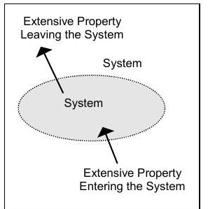
Figure \(\PageIndex{1}\): System-surroundings interactions are represented as transfers of an extensive property.

2.2.1 Rate Form of the Accounting Concept

The most general form of the accounting concept we will use is the rate form. This form is valid at any instant in time. The rate-form of the accounting principle for an extensive property (EP) can be written in words for any system:

Rate-Form Accounting Principle for an Extensive Property

The rate of accumulation of EP inside the system at time \(t\) equals the rate of transport of EP into the system at time \(t\) minus the rate of transport of EP out of the system at time \(t\) plus the rate of generation (production) of EP inside the system at time \(t\) minus the rate of consumption (destruction) of EP inside the system at time \(t\).

In an equation-like format, the words can be presented as

Figure \(\PageIndex{2}\): The rate-form accounting principle for an extensive property expressed in words in the form of an equation.

If we let the symbol \(B\) represent a generic extensive property, we can write this more compactly in symbols:

\[ \frac{d}{dt} \underbrace{ B_{sys} } _{B \text{ inside the system} } = \underbrace{ \{ \dot{B}_{in} - \dot{B}_{out} \} } _{ \text{Transport of } B \text{ inside the system} } + \underbrace{ \{ \dot{B}_{gen} - \dot{B}_{cons} \} } _{\text{Generation/Consumption of } B \text{ inside the system} } \nonumber \]

Please note that all of the terms in this equation are defined independently of the accounting concept. The accounting concept gains its power from its ability to relate these various terms for any system.

The rate-form of the accounting equation, Eq. \(\PageIndex{1}\), can be written in even a more compact form if we introduce the idea of net transport and net generation:

\[ \begin{align} \frac{d}{dt} \underbrace{ B_{sys} } _{B \text{ inside the system} } &= \underbrace{ \{ \dot{B}_{in} - \dot{B}_{out} \} } _{ \text{Transport of } B \text{ inside the system} } + \underbrace{ \{ \dot{B}_{gen} - \dot{B}_{cons} \} } _{\text{Generation/Consumption of } B \text{ inside the system} } \nonumber \\ &= \quad \dot{B}_{in, net} + \dot{B}_{gen, net} \end{align} \nonumber \]

In this notation, the first term on the right-hand side is positive if there is more transport into the system than out of the system. A negative value indicates that there is more leaving the system than entering.

Test Yourself

The graph below shows \(B_{sys}\) as a function of time for a system.

(a) How you could use this graph to explain the meaning of the term \(\frac{dB_{sys}} {dt}\)?

(b) Where is \(B_{sys}\) increasing? Decreasing?

(c) Where is \(\frac{dB_{sys}} {dt}\) positive? Negative?

(d) How are your answers to parts (b) and (c) related?

Because mathematics is the primary language for our analysis and a convenient short-hand for communicating our ideas, it is important to clearly understand what the various symbols and notation means. Starting with Eq. \(\PageIndex{1}\) and \(\PageIndex{2}\), it is very important to recognize that the left-hand side and right-hand side of each of these equations represent different things. The left-hand describes what is happening inside the system and describes how the amount of extensive property \(B\) is increasing or decreasing inside the system. The right-hand side describes something about how much of extensive property \(B\) is crossing the system boundary or is being consumed or generated inside the system.

Physically, the derivative on the left-hand side of Eq. \(\PageIndex{1}\) and \(\PageIndex{2}\) represents the rate of change or accumulation of the extensive property \(B_{sys}\) inside the system at any time \(t\). It is the rate of change of something that is contained inside the system, \(B_{sys}\). Please note that it is just an ordinary derivative. Mathematically this is correct because the amount of the extensive property \(B\) inside the system, \(B_{sys}\), is only a function of time, i.e. \(B_{sys} (t)\). The ordinary derivative of \(B_{sys}\) with respect to time, \(dB_{sys} / dt\), represents the rate of change of \(B\) inside the system.

If I had a graph showing the amount of \(B\) inside the system as a function of time, then \(dB_{sys} / dt\) represents the slope of the line at any desired time. To evaluate this derivative, I must keep track of all the \(B\) inside the system as a function of time. To determine the rate of change of \(B_{sys}\), I must be able to calculate the ordinary derivative or relate this term to other measurable quantities.

Mathematically, the terms on the right-hand side of Eq. \(\PageIndex{1}\) and \(\PageIndex{2}\) are not derivatives. As used here, the dot above a symbol does not represent differentiation. The "dot-above" notation, \(\dot{B}\), represents a transport rate, an interaction, between the system and its surroundings where \(B\) flows across the system boundary or the rate at which \(B\) is produced or consumed inside the system. Let me repeat this once again for emphasis: \(\dot{B}\) is not a derivative.

What is it, then? "\(B\) with a dot above it" or "\(B\) dot," \(\dot{B}\), does not represent a rate of change of anything inside the system. It represents the rate at which the extensive property \(B\) is being transported across the boundary of a system or generated (or consumed) inside a system. In theory, knowledge about \(\dot{B}\) is unrelated to the amount of \(B\) inside the system. (Yeah, yeah, yeah! I know that it can be related to what is inside the system through the accounting principle, but that's the whole point. \(\dot{B}\) and \(dB_{sys} / dt\) are two different things that are defined and can be measured independently of each other. The accounting concept shows us how they can be related to each other.)

Example — Who's Eating the Crackers?

Let's take a simple example to try and understand the differences. Assume your mom buys you a box of animal crackers. (Who doesn't love animal crackers?) As soon as you get the box, you start eating the animal crackers. Your jealous younger brother and sister start keeping track of the crackers to see if they will get any.

Your brother is pretty active and has a hard time sitting still, so every five minutes your brother runs back in the room, yanks the box away from you, and counts the number of crackers in the box. Then he runs away and doesn't see you eat the crackers. To help him remember, he writes these numbers down as a table showing the number of crackers in the box at five-minute intervals, i.e. at 0, 5, 10 min, etc.

Your sister, on the other hand, is much less combative. She watches you eat the crackers and just counts how many crackers you take out of the box during each 5 minute interval, 0 min to 5 min, 5 min to 10 min, etc. Unfortunately, your siblings don't get along either so they do not share information with each other.

The results of their efforts are shown below in the table.

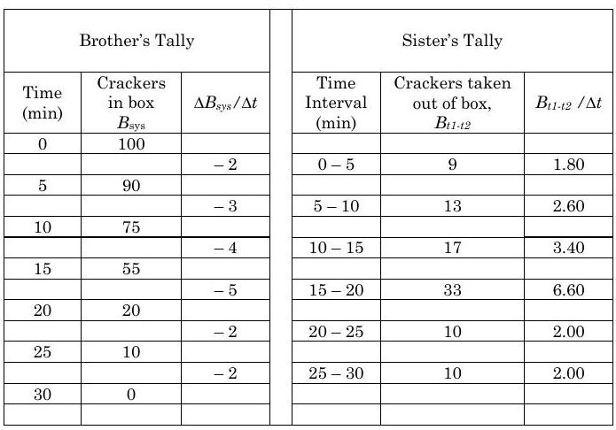
If the number of crackers in the box is called \(B\) then your brother can plot a graph that shows a series of points from the function \(B_{sys}(t)\) for the box. He can use this information to calculate the average rate of change for any interval using the formula \( (dB_{sys} / dt) _{average} = \Delta B / \Delta t\) for any 5-minute interval. Notice that all he has to know to compute the rate of change is how many crackers are in the box as a function of time. Unfortunately, your brother has no idea where the crackers are going unless he sees you take them out.

Now your sister has no idea how many crackers are in the box, but she has sufficient information to compute the average transport rate of crackers out of the box (how many you ate per minute). She does this by dividing the number of crackers you took out in one five-minute interval, say \(B_{0-5}\), and dividing it by the time interval, 5 minutes, i.e., \(\dot{B}_{out, average} = B_{0-5} / \Delta t\). Notice that all your sister needed to calculate the rate of transport out of the box was to focus on the boundary of they system (the box) and count how many crackers crossed it in any give time period. This is not a derivative of anything; it is a transport rate, but not a derivative. She knows the average rate at which crackers were transported out of the box, but she knows nothing about the rate of change of crackers inside the box.

Your sister and brother get so intrigued with their measurements that they totally forget to eat any crackers; however, they do decide to compare their information. Much to their surprise, they discover the following:

\[ \left( \frac{dB_{sys}}{dt} \right) _{average} \neq - \dot{B}_{out, average} \nonumber \]

The average rate of change of crackers inside the box did not equal the average transport rate of crackers out of the box. What happened?

Well, it seems that someone forgot to notice the small mouse in the box that was consuming crackers at the average rate of \(\dot{B}_{mouse, average}\). If we account for the mouse eating (consuming) the crackers we see that

\[ \left( \frac{dB_{sys}}{dt} \right) _{average} = - \dot{B}_{out, average} - \dot{B}_{mouse, average} \nonumber \]

should apply to this system. This equation could be used to solve for the average consumption rate at which the mouse ate the crackers.

Several things can be learned from this example.

• All of the terms in the accounting equation above have independent definitions and, under the best circumstances, could be measured directly.
• These terms can also be related through the accounting principle applied to the appropriate system (the box) for the appropriate property (number of crackers in the box), and the accounting principle can be used to solve for one unknown term.
• The only term that can be considered a derivative is the term on the left-hand side. The transport and consumption rates on the right-hand side are not derivatives and have no direct relationship to the rate of change of \(B\) inside the system except through the accounting concept applied correctly to a system.
• The accounting equation is most useful when we can say something a priori about the consumption and generation terms. If we had known that the box was mouse-free, we would only need to observe the transport rate of cookies out of the system to predict the rate of change of cookies inside the system. As we will show shortly, many important physical laws have attained this status precisely because empirical evidence allows us to say something about the consumption and generation terms.

Another way to understand the distinction between \(dB/dt\) and \(\dot{B}\) is to consider what happens when each is integrated over a time interval. When \(B\) with a dot over it is multiplied by \(dt\), the result is not the standard differential \(dB\) but a new symbol \(\delta B\) that represents not a "change in" but a "small amount of":

\[ \begin{align*} \delta B &= \dot{B} dt \\ &= \text{small amount of B} \\ &= \text{an inexact differential because } B \text{ is not a single-valued function of } t. \end{align*} \nonumber \]

On the other hand, you will recall from your calculus that the interpretation of the derivative \(dB/dt\) is

\[ dB = \frac{dB}{dt} dt \quad\quad \text{because } \frac{dB}{dt} = \lim_{\Delta t \to 0} \frac{B(t + \Delta t) - B(t)}{\Delta t} \nonumber \]

where \(dB\) equals "a small change" in \(B(t)\), a single-valued function.

Now the integral of the ordinary derivative with respect to time is the change in \(B\) between the two times:

\[ \int\limits_{t_1}^{t_2} \frac{dB}{dt} \, dt = \int\limits_{B(t_1)}^{B(t_2)} dB = B(t_2) - B(t_1) = \Delta B \nonumber \]

The integration of \(\dot{B}\) with respect to time over the same time interval is an amount of \(B\), not a change in \(B\), as shown below:

\[ \int\limits_{t_1}^{t_2} \dot{B} \, dt = \int\limits_{t_1}^{t_2} \delta B = B_{t_1 \to t_2} \nonumber \]

Take care to be sure that you understand the differences between these last two equations and that you can perform these integrations.

2.2.2 Finite-time (Integrated) Form of the Accounting Concept

There are many times when we are interested in a system that has undergone a process over a specified time interval. In these cases, it is possible to integrate the rate form to obtain a finite time form. Figure \(\PageIndex{5}\) shows a picture that is helpful for interpreting the finite-time form of the accounting concept. As you can see, the system exists in two different states and is connected by a process.

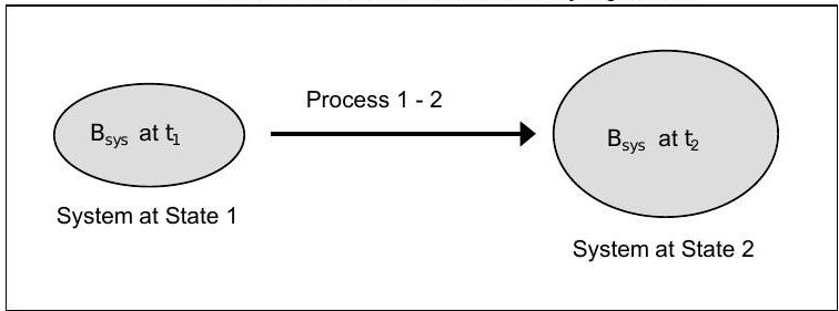
Figure \(\PageIndex{5}\): System undergoing a process from State 1 to State 2

In words, the finite-time form of the accounting concept is written as follows:

Figure \(\PageIndex{6}\): The finite-time form of the accounting concept expressed in words in the form of an equation.

In symbols, the finite-time form is written as follows:

\[ \begin{align} B_{sys} (t_2) - B_{sys} (t_1) &= \{ B_{in} - B_{out} \} + \{ B_{gen} - B_{cons} \} \nonumber \\ \Delta B_{sys} &= B_{in, net} + B_{gen, net} \end{align} \nonumber \]

The meaning of each of these symbols can be determined by comparison with the word statement.

Test Yourself

Now test yourself. Starting with Eq. \(\PageIndex{2}\) and using the results from Eq. \(\PageIndex{3}\) and \(\PageIndex{4}\), show the steps to develop Eq. \(\PageIndex{5}\).