
4.5: Simple Resistive Circuits
- Page ID
- 81492

The only circuits we will study in this course are simple resistive circuits that satisfy the lumped circuit model. Subsequent courses, especially ES 203 - Electrical Systems, will introduce you to the more complicated circuits and more complete solution techniques of circuit theory.
Simple resistive circuits are constructed of resistors and current and voltage sources. A current source is a circuit element that maintains a specified current independent of the voltage change across its terminals. A voltage source is a circuit element that maintains a specified voltage difference across its terminals independent of the current flowing through the element. The junction where two or more circuit elements meet is called a node. The voltage at a node is called a node voltage.
The brute-force approach in solving a simple resistive circuit is to identify each node as a system and apply the conservation of charge to each system. In the circuit theory language, we would say "apply Kirchhoff's current law to each node." For \(N\) nodes, this should provide \(N\) independent equations to solve for \(N\) unknowns. If additional information is required, you can introduce node voltages using Ohm's Law to relate the branch current through a resistor to the resistance and the differences in node voltages across the resistor. Sometimes this process can be shortened by applying conservation of charge to larger systems that include several nodes. However, there is not a single node voltage for the system.
A simple algorithm is given here for solving simple resistive circuits that satisfy the lumped circuit model. Although it is not always the quickest approach, it will almost always lead you to an answer by brute force. In fact, you will learn other methods later. (In later courses on circuit analysis you will learn that this approach is called nodal analysis.) We will restrict our attention here to simple resistive circuits composed of current sources, voltage sources, and resistors. The following algorithm makes use of Kirchhoff's current law (conservation of charge for lumped circuits) and Ohm's law.
Solving Simple Resistive Circuits using Conservation of Charge and Ohm's law
- Identify and label all nodes and branch currents. Nodes have a single voltage and at least one current input and one current output. Be sure to indicate the direction of the current in each branch of the circuit. Branches connect nodes and for our purposes a branch will consist of a resistor, a voltage source, or a current source.
- Apply conservation of charge (Kirchhoff's current law) to each node to relate the branch currents entering and leaving the node. (Recall that by definition, a node cannot accumulate charge.) Applying Kirchhoff's current law to a circuit with \(N\) nodes results in at most \(N\) independent equations relating the branch currents in the circuit. If the entire circuit can be included in a system with no charge flowing across the system boundary, only \(N-1\) independent equations can be obtained from applying KCL to the \(N\) nodes.
- Apply the appropriate constitutive relationship to describe the behavior of each branch.
- Resistors - Relate the voltage drop across each resistance to the current flowing through the resistance using Ohm's resistance model. It is critical that your voltage drop correspond with the assumed direction of the current in a resistor. By definition, \(i = \left( V_{in} - V_{out} \right) / R\) where the current flows into the resistor at a voltage \(V_{in}\) and leaves the resistor at a voltage \(V_{out}\).
- Voltage Sources - Specified voltage difference with no constraint on the direction or magnitude of the branch current
- Current Source - Specified current direction and magnitude for the branch with no constraint on the voltage difference across the branch.
(Note that even though we call these sources, they are not generating charge within our system. It would be more correct to think of current and voltage sources as being charge movers with no charge storage.)
- Select one node as the zero point and arbitrarily set its voltage value to zero. This is typically the grounded node. (For our purposes, we will assume that there is no current flowing into or out of ground. The existence of ground loops with non-zero current flowing often occurs in real systems; however, we will assume that our circuits are correctly grounded.) All node voltages are then defined with respect to this zero node.
- Check to see if you have sufficient equations to handle the number of unknowns. If you have followed this procedure a system with \(N\) nodes and \(B\) branches will have at most \(N+B\) unknowns: \(N\) node voltages and \(B\) branch currents. The actual number of unknowns is reduces by the known voltages (including ground) and currents specified for the circuit.
- Solve for the unknowns. (Matrix algebra can be a real time saver for large problems especially where there is a simple pattern for setting up the equations. For small systems of equations, it may be quicker to just set up the equations and let MAPLE or Mathematica solve them directly. The preferred method usually depends upon your familiarity with the software and how easily you can set up the matrices.)
- Check your answers. One approach is to examine a system that contains several nodes and then check to see that conservation of charge is satisfied.
The following example shows how to apply this technique to a simple resistive circuit that includes both a voltage source and a current source.
Find the unknown branch currents and node voltages in the circuit shown in the figure.
.png?revision=1&size=bestfit&width=775&height=472)
Figure \(\PageIndex{1}\): Circuit diagram for a circuit with 6 nodes, 1 battery, 5 resistors, and one known branch current.
Solution
Strategy \(\rightarrow\) This is clearly a circuit problem and will require application of conservation of charge along with suitable constitutive relationships.
First step is to label and locate all the nodes and branches. This gives
6 nodes: \(V_{1}, V_{2}, V_{3}, V_{4}, V_{5,} V_{6}\)
7 branches: \(i_{a}, i_{b}, i_{c}, i_{d}, i_{e}, i_{f}, i_{g}\)
.jpg?revision=1)
Figure \(\PageIndex{2}\): Circuit diagram from above with all nodes and branch currents marked and labeled.
Writing conservation of charge for each node assuming no charge accumulation (lumped circuit assumption), we get six equations relating the currents:
\[ \begin{align*} &\text{Node 1:} \quad 0 =i_{g} - i_{a} \quad\quad &\text{Node 4:} \quad 0=i_{d}-i_{c} \\ &\text{Node 2:} \quad 0=i_{a}+i_{b}-i_{e} \quad\quad\quad\quad &\text{Node 5:} \quad 0=i_{e}-i_{f}-i_{e} \\ &\text{Node 3:} \quad 0=i_{c}-i_{d} \quad \quad &\text{Node 6:} \quad 0=i_{f}-i_{g} \end{align*} \nonumber \]
Note that we have assumed no current in the ground connection. Also note that only five of these six equations are independent equations.
Now we can write the branch equations by using the appropriate constitutive relations:
\[ \begin{align*} & \text {Branch a: } \quad \left(V_{1}-V_{2}\right)=(3 \ \Omega) i_{a} \quad\quad \text { Branch e: } \quad\left(V_{2}-V_{5}\right)=(5 \ \Omega) i_{e} \\ & \text {Branch b: } \quad \left(V_{3}-V_{2}\right)=(2 \ \Omega) i_{b} \quad\quad \text { Branch f: } \quad \left(V_{5}-V_{6}\right)=(1 \ \Omega) i_{f} \\ & \text {Branch c: } \quad \left(V_{4}-V_{3}\right)=(1 \ \Omega) i_{c} \quad\quad \text { Branch g: } \quad i_{g}=4 \mathrm{~A} \\ & \text {Branch d: } \quad V_{5}-V_{4}=50 \text { volts } \end{align*} \nonumber \]
All seven of the branch equations are independent.
We now have 13 unknowns and 12 equations (5 node and 7 branch). The remaining equation comes from assigning the ground voltage to node 6.
\[ V_6 = 0 \nonumber \]
We should now have sufficient information to solve for the remaining voltages and currents. This is most easily done use a software package, e.g. MAPLE™ or EES.
MAPLE Solution:
There are 6 nodes in this problem (numbered 1,2,3,4,5,6). If we write conservation of charge for each node we will get 6 equations that relate the 6 unknown currents in the circuit:
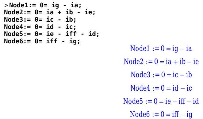
Figure \(\PageIndex{3}\): Code in MAPLE to set up equations relating conservation of charge for each node to the circuit currents.
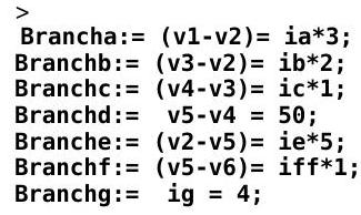
Now writing the 7 branch equations:
.jpg?revision=1)
Figure \(\PageIndex{4}\): Code in MAPLE to set up equations for voltage drop in each branch of the circuit, based on constitutive relations.
There are 7 branch currents and 6 node voltages. Unfortunately only 5 of the 6 conservation of charge relations are independent, so we need an additional constraint. The remaining constraint is supplied by establishing a ground node with zero potential. Based on the circuit schematic this node should probably be Node 6.
.png?revision=1&size=bestfit&width=721&height=67)
Figure \(\PageIndex{5}\): Code in MAPLE to assign a value of 0 to the ground node (node 6).
Now we can collect 12 independent equations to solve for the 6 currents and the 6 voltages.
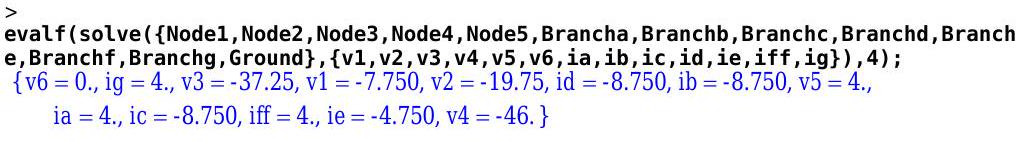
Figure \(\PageIndex{6}\): Code to solve for the problem variables, using 5 of the conservation of charge equations, and the numerical solutions returned by the program.
To check our solutions, let's try some variations and see what happens. If any 5 of the conservation of charge equations work then we ought to be able to solve with a different set. Let's try for a couple of cases. First, let's try using Node 6 instead of Node 1:
.jpg?revision=1)
Figure \(\PageIndex{7}\): Code to solve for the problem variables, using another set of 5 of the conservation of charge equations, and the numerical solutions returned by the program.
Now let's try using all of the nodes except Node 5:
.png?revision=1&size=bestfit&width=1145&height=146)
Figure \(\PageIndex{8}\): Code to solve for the problem variables, using another set of 5 of the conservation of charge equations, and the numerical solutions returned by the program.
Looks OK. Now let's see what happens if we don't include the GROUND condition and don't put \(v_6\) in the variable list:
.png?revision=1&size=bestfit&width=1148&height=157)
Figure \(\PageIndex{9}\): Code from Figure \(\PageIndex{8}\) with \(v_6\) omitted from the variable list and the GROUND condition omitted from the conditions list, and the solutions returned by the program. All voltage solutions are in terms of \(v_6\).
Now let's try and see what happens if we just accidentally don't include the GROUND condition but we do include v6 in the variable list:
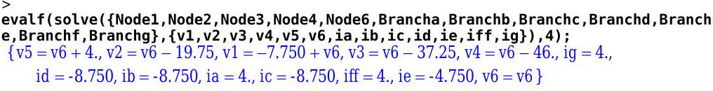
Figure \(\PageIndex{10}\): Code from Figure \(\PageIndex{8}\) with the GROUND condition omitted from the conditions list, and the solutions returned by the program. All voltage solutions are in terms of \(v_6\).
Notice how all the voltages include a \(v_6\) component. What does this mean?
Finally, what happens if we just leave out the variables list?
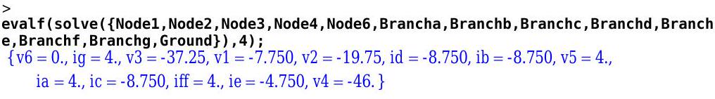.jpg?revision=1)
Figure \(\PageIndex{11}\): Code from Figure \(\PageIndex{8}\) with the variables list removed, and the numerical solutions returned by the program.
Same answers, just in a different order.