
6.1: Why is this thing turning?
- Page ID
- 81499

Anyone who has changed a flat tire, used a wrench, thrown a Frisbee, hung on a tree limb, or pushed a large box knows something about the tendency for objects to rotate or resist rotation. Angular momentum is the extensive physical property related to this phenomenon. Before we can develop the conservation of angular momentum relation, we must introduce several concepts for describing angular motion and the moment of a force.
What's the purpose of a "cheater" bar applied to a wrench? (A "cheater" bar is a piece of pipe slipped over the end of a wrench to extend its length.)
Where is the best place to push a filing cabinet on rollers? How did you judge best?
To refresh your memory, imagine that your car has a flat tire and you must change it (See Figure \(\PageIndex{1}\)). To change the tire, you first raise the tire off the ground using a car jack. Next, you place the tire iron on a lug nut and try to loosen it. In the sketch, the force \(\mathbf{F}\) acts on the tire iron at point \(P\), the axle of the tire is at point \(O\), and the nut is located at point \(N\).
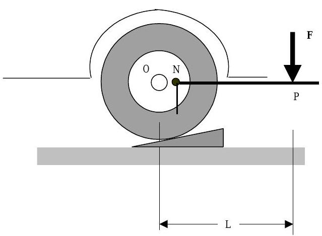
Figure \(\PageIndex{1}\): Changing a tire.
If you have been lucky in life, you may be a novice at tire changing, and will discover that the tire rotates when you push on the tire iron. A driver with less luck and more experience changing tires might only raise the tire partially or insert a wedge to prevent the tire from rotating. Experienced tire changers know that our ability to loosen the nut depends on both the force \(\mathbf{F}\) and its point of application (point \(P\)). They also know that the effectiveness of the applied force \(\mathbf{F}\) is less if it is applied at an angle to the tire iron.
What would happen if the force was applied at point \(N\)? Would you be able to loosen the nut? Would the tire turn?
6.1.1 Moment of a force about a point
To quantify the ability of the force to rotate the tire we need a physical quantity that accounts for the magnitude and direction of force \(\mathbf{F}\) as well as its point of application. The quantity we desire is the moment of a force about a point.
The moment of a force \(\mathbf{F}\) about a point \(\bf{O}\) is the vector (or cross) product of the position vector \(\mathbf{r}\) and the force \(\mathbf{F}\):
\[ \mathbf{M}_O = \mathbf{r} \times \mathbf{F} \nonumber \]
where \(\mathbf{r}\) is the position vector that extends from the point \(O\) to the point of application of the force (See Figure \(\PageIndex{2}\)).
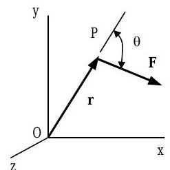
Figure \(\PageIndex{2}\): Calculating moment of a force \(\mathbf{F}\) about a point \(O\).
When the position vector \(\mathbf{r}\) and the force vector \(\mathbf{F}\) are written in terms of their components as \[\mathbf{r} = x \mathbf{i}+y \mathbf{j}+z \mathbf{k} \quad \text { and } \quad \mathbf{F}=F_{x} \mathbf{i}+F_{y} \mathbf{j}+F_{z} \mathbf{k} \nonumber \] Eq. \((\PageIndex{1})\) is evaluated as the follows using standard cross-product operations: \[\begin{align} \mathbf{M}_{o} &=\mathbf{r} \times \mathbf{F}=\left| \begin{array}{ccc} \mathbf{i} & \mathbf{j} & \mathbf{k} \\ x & y & z \\ F_{x} & F_{y} & F_{z} \end{array}\right| \nonumber \\[4pt] &=\mathbf{i}\left|\begin{array}{cc} y & z \\ F_{y} & F_{z} \end{array}\right|-\mathbf{j}\left|\begin{array}{cc} x & z \\ F_{x} & F_{z} \end{array}\right|+\mathbf{k}\left|\begin{array}{cc} x & y \\[4pt] F_{x} & F_{y} \end{array}\right| \\ &=\left(y F_{z}-z F_{y}\right) \mathbf{i}-\left(x F_{z}-z F_{x}\right) \mathbf{j}+\left(x F_{y}-y F_{x}\right) \mathbf{k} \nonumber \end{align} \nonumber \]
If we restrict ourselves to motion in the \(x \text{-} y\) plane (plane motion), the only component of \(\mathbf{M}_O\) with a non-zero value is the \(z\)-component — the last term on the right-hand side of Eq. \((\PageIndex{3})\).
From our knowledge of vectors, we can say several things about this result:
- The position vector \(\mathbf{r}\) and the force vector \(\mathbf{F}\) lie in a plane.
- The moment \(\mathbf{M}_O\) of the force \(\mathbf{F}\) about point \(O\) is a vector (see Eq. \((\PageIndex{3})\)).
- The line of action of the moment vector \(\mathbf{M}_{O}\) is normal (perpendicular) to the plane that contains both \(\mathbf{r}\) and \(\mathbf{F}\).
- The point of application of the moment vector \(\mathbf{M}_{O}\) is at point \(O\), the point about which we are taking the moment.
- The sense of the direction of the moment \(\mathbf{M}_{O}\) and the sense of the rotation it could impart can be described by the right-hand rule in several ways (See Figure \(\PageIndex{3}\)):
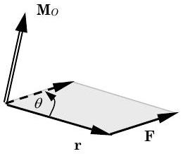
Figure \(\PageIndex{3}\): Sense of direction of \(\mathbf{M}_O\) using the right-hand rule. - Align the fingers of your right hand in the direction of the position vector \(\mathbf{r}\) and curl them in the direction of the force \(\mathbf{F}\). Your thumb now points in the direction of the moment \(\mathbf{M}_{O}\) and your fingers curl to show the sense of rotation for the moment \(\mathbf{M}_{O}\).
- Imagine sliding vector \(\mathbf{r}\) or \(\mathbf{F}\) until they are tail-to-tail. Align the fingers of your right hand in the direction of the position vector \(\mathbf{r}\) and curl your fingers in the direction of force \(\mathbf{F}\). Your curled fingers now indicate the sense of rotation for the moment \(\mathbf{M}_{O}\) and your thumb points in the direction of moment \(\mathbf{M}_{\text {O}}\).
- Curl the fingers of your right hand and point the thumb of your right hand in the direction of moment \(\mathbf{M}_{O}\). The direction your fingers curl is the sense of rotation for the moment \(\mathbf{M}_{O}\).
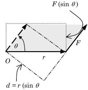
- The magnitude of the moment vector \(\mathbf{M}_{O}\) is the square root of the dot product of \(\mathbf{M}_{O}\) with itself and is calculated as follows: \[\begin{array} M M_{O} &=\left|\mathbf{M}_{o}\right|=\left(\mathbf{M}_{O} \cdot \mathbf{M}_{O}\right)^{1 / 2} \\ &=\left[\left(y F_{z}-z F_{y}\right)^{2}+\left(x F_{z}-z F_{x}\right)^{2}+\left(x F_{y}-y F_{x}\right)^{2}\right]^{1 / 2} \end{array} \nonumber \] It can also be calculated using the relationship \[M_{o}=\left|\mathbf{M}_{o}\right|=|\mathbf{r}||\mathbf{F}| \sin \theta=r F(\sin \theta) \nonumber \] where \(\theta\) is the angle between the lines-of-action of vectors \(\mathbf{r}\) and \(\mathbf{F}\) and is measured as though \(\mathbf{r}\) and \(\mathbf{F}\) were placed tail-to-tail. A positive angle satisfies the right-hand rule as described above. Eq. \(( \PageIndex{5})\) can be interpreted as the area of a parallelogram formed by the vectors \(\mathbf{r}\) and \(\mathbf{F}\) (See Figure \(\PageIndex{4}\)).
.jpg?revision=1)
Figure \(\PageIndex{4}\): Interpreting the magnitude of \(\mathbf{M}_O\) as an area. Two additional rectangles shown in Figure \(\PageIndex{4}\) have areas equal in magnitude to the shaded area. The rectangle of length \(d_{\perp}\) and width \(F\) has an area of \[\begin{align} M_{O} &=(r \sin \theta) F \nonumber \\ &=d_{\perp} \times F \quad=\underbrace{\left[\begin{array}{c} \text { Shortest distance } \\ \text { between point } O \\ \text { and the line-of-action } \\ \text { of force } \mathbf{F} \end{array}\right]}_{\text {Often called the "lever arm" }} \times\left[\begin{array}{c} \text { Magnitude } \\ \text { of } \\ \text { force } \mathbf{F} \end{array}\right] \end{align} \nonumber \] The rectangle of length \(r\) and width \(F \sin \theta\) has an area of \[\begin{align} M_{O} &=r(F \sin \theta) \nonumber \\ &=r \times F_{\perp}=\left[\begin{array}{c} \text { Magnitude } \\ \text { of the } \\ \text { position vector } \mathbf{r} \end{array}\right] \times\left[\begin{array}{c} \text { Component of force } \mathbf{F} \\ \text { that is } \perp \text { to } \\ \text { the line-of-action of } \mathbf{r} \end{array}\right] \end{align} \nonumber \] For most cases with two-dimensional (plane) motion, you will find that using Eqs. \((\PageIndex{6})\) or \((\PageIndex{7})\) is much simpler than using the formal cross product mathematics.
For each of the following two-dimensional cases, determine the magnitude and direction [Clockwise (CW) or counter-clockwise (CCW)] of the moment of force \(\mathbf{F}\) about point \(O\):
a)
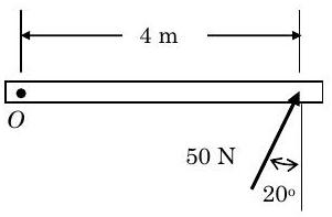
Figure \(\PageIndex{5}\): A force is applied at an angle to one end of a bar.
b)
.jpg?revision=1)
Figure \(\PageIndex{6}\): A force is applied at an angle to one end of a bar.
c)
.jpg?revision=1)
Figure \(\PageIndex{7}\): A force is applied at an angle to one end of a rigid body.
- Answer
-
a) \(187.9 \ \mathrm{N} \cdot \mathrm{m CCW}\)
b) \(34.73 \ \mathrm{N} \cdot \mathrm{m CW}\)
c) \(176.8 \ \mathrm{N} \cdot \mathrm{m CCW}\)
6.1.2 Moment of a force couple
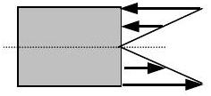
There is a special type of external force system called a force couple. A force couple consists of two external forces that have equal magnitude, parallel lines-of-action, and opposite sense (See Figure \(\PageIndex{8}\)). Thus, a force couple results in a zero net force on a system. Or stating this another way, a force couple transfers zero linear momentum to a system. However, a quick examination of the figure shows that the force couple does in fact attempt to turn or rotate the system.
.png?revision=1)
Figure \(\PageIndex{8}\): A force couple.
The moment of a force couple about point \(O\) can be calculated with reference to Figure \(\PageIndex{8}\) as follows: \[ \begin{align} \mathbf{M}_{O, \text { couple }} &= \mathbf{M}_{O, \ F_{1}} + \mathbf{M}_{O, \ F_{2}} \nonumber \\ &= \left( \mathbf{r}_{1} \times \mathbf{F}_{1} \right) + \left( \mathbf{r}_{2} \times \mathbf{F}_{2}\right) \quad\quad\quad \text { where } \left| \mathbf{F}_{1} \right| = \left|\mathbf{F}_{2}\right| = F \nonumber \\ &= \left[ \left( d_{\perp, 1} \times F_{1}\right) \,\, \mathrm{CCW} \right] + \left[ \left( d_{\perp, 2} \times F_{2}\right) \,\, \mathrm{CW} \right] \\ & = \left[ -\left( d_{\perp, 1} \times F_{1}\right) \quad + \quad \left(d_{\perp, 2} \times F_{2}\right) \right] \quad \text { CW } \nonumber \\ &= d \times F \quad \text { CW } \quad\quad\quad\quad\quad\quad\quad \text { where } d=\left| d_{\perp, 1}-d_{\perp, 2}\right| \nonumber \\ {} \nonumber \\ \mathbf{M}_{O, \text { couple }} &= d \times F \text{ in a CW direction} \nonumber \end{align} \nonumber \]
Note that if we had calculated the moment of the force couple shown in Figure \(\PageIndex{8}\) about point \(O'\) or point \(O''\) we would have found exactly the same result. Thus, the moment of a couple does not seem to be tied to a particular point, unlike what we found with the moment of a force about a point.
We can say the following about a force couple with force \(\mathbf{F}\) and a distance \(d\) separating the forces' lines of action:
- The lines of action of the two forces in a force couple lie in the same plane.
- A force couple transfers no net linear momentum to a system.
- The moment produced by a force couple is a vector \(\mathbf{M}_{\text {couple}}\).
- The line of action of the moment vector \(\mathbf{M}_{\text {couple}}\) is normal (perpendicular) to the plane that contains the force couple.
- The point of application of the moment vector \(\mathbf{M}_{\text {couple}}\) can be at any point in the plane of the couple. Because the point of application is free to move, this type of vector is sometimes called a free vector.
- The sense of the moment vector \(\mathbf{M}_{\text {couple can be obtained from ob. }}\) serving the direction of rotation the force couple could impart. The direction of the moment vector can be found by curling the fingers of your right hand to match the sense of the force couple and aligning your thumb along the line of action. Your thumb now points in direction for the moment vector \(\mathbf{M}_{\text {couple. }}\).
- The magnitude of the moment vector \(\mathbf{M}_{\text {couple is equal to the product }}\) of the magnitude of one of the force vectors and the shortest distance between the lines of action, \(d\): \[M_{\text {couple}} = \left| \mathbf{M}_{\text {couple}}\right| = d \times |\mathbf{F}| = d \times F \nonumber \]
We will frequently encounter systems where the force distribution on some portion of the boundary looks like that shown in Part (a) of Figure \(\PageIndex{9}\). On the upper half of the boundary, the forces are compressive (they push on the system), and on the lower half of the boundary, the forces are tensile (they pull on the system). If every force on the upper half has a mirror image of opposite sense on the lower half, this distribution represents a couple and the net force on the boundary is zero; however there is a net moment due to the couple as shown in Part (b) of Figure \(\PageIndex{9}\). There will also be occasions where the force distribution on the boundary is actually the sum of a couple and a net force.
 a) Distributed couple acting on the boundary
.png?revision=1)
b) Equivalent moment due to distributed couple
Calculate the magnitude and the direction (CW or CCW) for the net moment about the point \(O\) :
.jpg?revision=1)
Figure \(\PageIndex{10}\): Point forces and a force couple are applied to a curved shape.