7.1: Mechanics and the Mechanical Energy Balance

Historically, the general conservation of energy principle was one of the last principles identified by the scientific community. However, restricted forms of the principle were derived earlier from other fundamental principles. One of the most useful of these is the mechanical energy balance. In this section, we will demonstrate how this balance can be developed from the conservation of linear momentum. Along the way, we will introduce several new concepts — such as mechanical work, mechanical power, and mechanical energy — that are rooted in the study of mechanics.

7.1.1 Mechanical Work and Mechanical Power

Early in our study of conservation of linear momentum we examined different ways to write the time rate of change of linear momentum for a particle: \[\frac{d}{d t}(m V) = m \frac{d V}{d t} = m \left(\frac{d V}{d x}\right) \left(\frac{d x}{d t}\right) = m\left[V \frac{d V}{d x}\right] \nonumber \] The motivation for this exercise was the need to integrate the linear momentum equation when information was only given as a function of only position \(x\). This same concern leads us to consider the integral of a force with position.

Mechanical Work

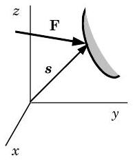
Figure \(\PageIndex{1}\): Surface force acting on the boundary of a system.

The mechanical work done by a surface force \(\mathbf{F}\) acting on the boundary of a system (see Figure \(\PageIndex{1}\)) is the integral \[W_{\text {mech}} \equiv \int\limits_{\mathbf{s}_{1}}^{\mathbf{s}_{2}} \mathbf{F} \cdot d \mathbf{s} = \int\limits_{1}^{2} \delta W_{\text {mech}} \quad \text { where } \delta W_{\text {mech}} \equiv \mathbf{F} \cdot d \mathbf{s} \nonumber \] where \(d \mathbf{s}\) is the differential displacement vector of the point of application of the force on the boundary and \(\mathbf{s}_{1}\) and \(\mathbf{s}_{2}\), respectively, are the initial and final positions of the boundary.

Figure \(\PageIndex{2}\): Evaluating differential mechanical work, \(\delta W_{\text {mech}}\).

To better understand this integral, it is useful to examine the differential amount of work \(\delta W_{\text {mech}}\). To help, Figure \(\PageIndex{2}\) shows both the force \(\mathbf{F}\) and the displacement \(d \mathbf{s}\). Note that force \(\mathbf{F}\) can be decomposed into two components: \(\mathbf{F}_{\perp}\) normal to \(d \mathbf{s}\) and \(\mathbf{F}_{\text {tan}}\) tangent to \(d \mathbf{s}\). Using the definition of a dot product between two vectors, we have the following result for \(\delta W_{\text {mech}}\):

\[ \begin{align} \delta W_{\text{mech}} &= \mathbf{F} \cdot d \mathbf{s} = |\mathbf{F}| |d \mathbf{s}| \cos \theta = F \cdot ds \cdot \cos \theta \nonumber \\[4pt] &= F \cdot \underbrace{ \left[ ds \cdot \cos \theta \right] }_{\begin{array}{c} \text{Component of displacement} \\ \text{that is parallel to the } \\ \text{force's line of action} \end{array}} = \underbrace{ \left[ F \cdot \cos \theta \right] }_{\begin{array}{c} \mathbf{F}_{\text{tan }} = \text{ Component of the force} \\ \text{that is parallel to the} \\ \text{displacement's line of action} \end{array}} \end{align} \nonumber \]

From Eq. \(\PageIndex{2}\) above, we see that there are two different interpretations for the differential amount of work. \(\delta W_{\text {mech}}\) can interpreted as (1) the product of the force and the component of the displacement that is parallel to the force or (2) the product of the displacement and the component of the force that is parallel to the displacement.

Several additional points about mechanical work can be discovered by a close examination of the integral, Eq. \(\PageIndex{1}\):

• Mechanical work is a scalar quantity; however, it is a signed quantity because the dot product \(\mathbf{F} \cdot d \mathbf{s}\) can be positive or negative depending on the angle \(\theta\) between the vectors (See Figure \(\PageIndex{2}\))
• The dimensions of mechanical work are \([\text{Force}] [\text{L}]\) or \([\text{M}] [\text{L}]^{2} [\text{T}]^{-2}\)
• The units for work are \(\text{N} \cdot \text{m}\) in SI and \(\text{ft} \cdot \text{lbf}\) in the USCS system. The fact that one set of units is force-length and the other is length-force is arbitrary and probably the result of what sounded good to the ear.
• The integral and hence mechanical work can only be evaluated if one knows the end states and the path of the process connecting these states. Mathematically, you must know \(\mathbf{F}\) as a function of position \(\mathbf{s}\) to evaluate the integral.
• Mechanical work for a system cannot be evaluated in a specific state or at a specific time. It can only be evaluated for a process — a change in state. Mechanical work is an example of a path function because its defining integral, Eq. \(\PageIndex{1}\), can only be evaluated when the path of the process is known. This is in contrast to, say, the problem of finding the change in volume for a process. To find the change in volume of a system, we need only know the system volume at the each end state without regard to the path of the process. Thus, volume, like all properties of a system, is a state (or point) function.

Test your understanding — What's the work?

(a) \(\mathbf{F}=F \mathbf{i} \quad\) and \(\quad \mathbf{s}=x \mathbf{i} + y \mathbf{j}\) where \(x=a t\) and \(y=b t\) from \(t_{1}\) to \(t_{2}\) \[\begin{aligned} W_{\text {mech}} &= \int\limits_{\mathbf{s}_{1}}^{\mathbf{s}_{2}} \mathbf{F} \cdot d \mathbf{s} = \int\limits_{1}^{2}(F \mathbf{i}) \cdot (d x \mathbf{i}+d y \mathbf{j}) = \int\limits_{1}^{2} \left[ \underbrace{ (F \mathbf{i}) \cdot(d x \mathbf{i}) }_{\mathbf{i} \cdot \mathbf{i}=1} + \underbrace{ (F \mathbf{i}) \cdot(d y \mathbf{j}) }_{\mathbf{i} \cdot \mathbf{j}=0} \right] \\ &= \int\limits_{x_{1}}^{x_{2}} F \ dx \quad \text { but } \quad dx =adt \\ &= \int\limits_{t_{1}}^{t_{2}}(F a) \ dt = F a\left(t_{2}-t_{1}\right) \end{aligned} \nonumber \] Note that even though the point of application moves in the \(\mathbf{j}\) direction, there is no component of the force \(\mathbf{F}\) in that direction and the only work is done by the component of the force in the \(\mathbf{i}\) direction.

(b) \(\mathbf{F}=F_{x} \mathbf{i}+F_{y} \mathbf{j} \quad\) and \(\quad \mathbf{s}=x \mathbf{i}+y \mathbf{j} \quad\) from \(\mathbf{s}_{1}\) to \(\mathbf{s}_{2} \quad\) if \(y=x^{2}\) \[\begin{aligned} W_{\text {mech}} &= \int\limits_{\mathbf{s}_{1}}^{\mathbf{s}_{2}} \mathbf{F} \cdot d \mathbf{s} = \int\limits_{1}^{2} \left(F_{x} \mathbf{i}+F_{y} \mathbf{j}\right) \cdot \left[ (dx)\mathbf{i} + (dy)\mathbf{j} \right] = \int\limits_{x_{1}}^{x_{2}} \underbrace{ \left[ \left(F_{x} \cdot d x\right) + \left(F_{y} \cdot d y\right)\right] }_{\mathrm{i} \cdot \mathbf{j} = \mathbf{j} \cdot \mathbf{i} =0 \text { and } \mathbf{i} \cdot \mathbf{i} = \mathbf{j} \cdot \mathbf{j} = 1} \\ &= \int\limits_{1}^{2} \left[\left(F_{x} \cdot d x\right) + \left(F_{y} \cdot \underbrace{d y}_{d y=2x \ dx}\right) \right] \\ &= \int\limits_{x_{1}}^{x_{2}} \left[F_{x} + \left(2x \cdot F_{y}\right)\right] \ dx = F_{x}\left(x_{2}-x_{1}\right) + F_{y} \underbrace{ \left(x_{2}^{\ 2} - x_{1}^{\ 2}\right) }_{=\left(y_{2}-y_{1}\right)} \end{aligned} \nonumber \]

Mechanical Power

The time rate at which surface force \(\mathbf{F}\) does work on the system is called the mechanical power and is defined by the equation \[\dot{W}_{\text {mech}} \equiv \mathbf{F} \cdot \mathbf{V} \nonumber \] where \(\mathbf{V}\) is the velocity of the point of application of the force \(\mathbf{F}\) on the boundary of the system.

By integrating the mechanical power with respect to time over a finite-time interval, we can demonstrate the relationship between mechanical power and mechanical work: \[\int\limits_{t_{1}}^{t_{2}} \dot{W}_{\text {mech}} \ dt = \left\{ \begin{array}{l} \int\limits_{t_{1}}^{t_{2}} (\mathbf{F} \cdot \mathbf{V}) \ dt = \int\limits_{t_{1}}^{t_{2}} \left(\mathbf{F} \cdot \frac{d \mathbf{s}}{d t}\right) \ dt = \int\limits_{t_{1}}^{t_{2}} \underbrace{\mathbf{F} \cdot d \mathbf{s}}_{\delta W_{\text{mech}}} = W_{\text {mech}} \\ \int\limits_{1}^{2} \delta W_{\text {mech}} = W_{\text {mech}} \quad \text { where } \quad \delta W_{\text {mech}}=\dot{W}_{\text {mech}} dt \end{array}\right. \nonumber \] Note that the integral of \(\delta W_{\text {mech}}\) does not equal \(\Delta W_{\text {mech}}\).

Several additional points should be made about mechanical power and its relation to mechanical work:

• Mechanical power, unlike mechanical work, can be evaluated at a specific time because it is the instantaneous rate at which work is being done.
• The dimensions for mechanical power are \([\mathrm{Force}][\mathrm{L}] /[\mathrm{T}]\) or \([\mathrm{M}][\mathrm{L}]^{2}[\mathrm{T}]^{-3}\).
• The units for mechanical power are \(\mathrm{N} \cdot \mathrm{m} / \mathrm{s}\) in SI and \(\mathrm{ft} \cdot \mathrm{lbf} / \mathrm{s}\) or \(\mathrm{hp}\) (horsepower) in USCS. (\(1 \mathrm{hp}=550 \mathrm{ft} \cdot \mathrm{lbf} / \mathrm{s}\), approximately).

Before leaving the discussion of mechanical work and mechanical power, please note that they have very precise definitions and can, given sufficient information, be evaluated from their defining equations. Now we investigate how our knowledge of mechanical power and work can help us solve some problems of mechanics using scalars instead of vectors.

7.1.2 The Work-Energy Principle

The work-energy principle is the direct link between the conservation of linear momentum and the mechanical energy balance. It is developed here first for a particle and then expanded to include a system of particles.

Work-Energy Principle for a Particle

Consider the motion of a particle of mass \(m\) in a gravitational field. (Recall that a particle is a system with its mass concentrated at a point that may only translate as it moves through space, i.e. its mass moment of inertia is zero.) As shown in Figure \(\PageIndex{3}\), the position vector \(\mathbf{s}\) describes the position of the particle. The only external forces acting on the particle are the weight \(\mathbf{W}\) and the net surface (or contact) forces \(\mathbf{R}\). Note that the gravity vector acts in the direction of the negative \(z\)-axis.

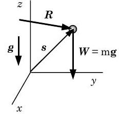
Figure \(\PageIndex{3}\): Motion of a particle in a gravitational field..

If we apply the conservation of linear momentum to the particle we have \[\frac{d \mathbf{P}_{\mathrm{sys}}}{dt} = \mathbf{R}+\mathbf{W} \quad \rightarrow \quad m \frac{d \mathbf{V}_{G}}{dt} = \mathbf{R}+m \mathbf{g} \nonumber \] where we have recognized that a particle is a closed system, its linear momentum is \(\mathbf{P}_{\text {sys}} = m \mathbf{V}_{G}\), and its weight is \(m \mathbf{g}\).

Now let us evaluate the mechanical power supplied to the particle by the contact force \(\mathbf{R}\). Since the particle is a point, the force \(\mathbf{R}\) moves with the velocity \(\mathbf{V}_{G}\) and the mechanical work is \[\dot{W}_{\text {mech}} = \mathbf{R} \cdot \mathbf{V}_{G} \nonumber \] To eliminate the surface force \(\mathbf{R}\), we use the results of the conservation of linear momentum, Eq. \(\PageIndex{5}\), as follows: \[\begin{array}{l} \dot{W}_{\text {mech}} &= \mathbf{R} \cdot \mathbf{V}_{G} = \left[m \dfrac{d \mathbf{V}_{G}}{dt} - m \mathbf{g}\right] \cdot \mathbf{V}_{G} \\ &= \underbrace{m \dfrac{d \mathbf{V}_{G}}{d t} \cdot \mathbf{V}_{G} }_{\text {Inertia term}} - \underbrace{m \mathbf{g} \cdot \mathbf{V}_{G}}_{\text {Gravitation Term}} \end{array} \nonumber \] We have identified an "Inertia term" and a "Gravitation term" on the right hand side of Eq. \(\PageIndex{7}\). Before continuing, we need to investigate these two terms.

The inertia term in Eq. \(\PageIndex{7}\) is the dot product of the particle velocity with the rate of change of the particle linear momentum. Starting with the inertia term and performing the dot product, we have

\[\begin{array}{l} \left[ \begin{array}{c} \text {Inertia} \\ \text {term} \end{array}\right] &= m \dfrac{d \mathbf{V}_{G}}{d t} \cdot \mathbf{V}_{G}=\dfrac{m}{2} \dfrac{d}{dt} \left(\mathbf{V}_{G} \cdot \mathbf{V}_{G}\right) \\ &= \dfrac{m}{2} \dfrac{d}{dt} \left(V_{G}{ }^{2}\right) = \dfrac{d}{dt} \left(m \dfrac{V_{G}{ }^{2}}{2}\right) = \dfrac{d E_{K}}{dt} \\ \text { where } E_{K} & \equiv m \dfrac{V_{G}{ }^{2}}{2}=\text { the kinetic energy of a particle } \end{array} \nonumber \]

Thus the inertia term is just the ordinary derivative of a scalar quantity we typically refer to as the kinetic energy of the particle. Because the kinetic energy only depends on properties of the system and also depends on the mass of the system, kinetic energy is an extensive property.

Similarly, we can massage the gravitation term. To do this, we refer back to Figure \(\PageIndex{3}\) and first write the velocity and the weight term using the unit vectors \(\mathbf{i}\), \(\mathbf{j}\), and \(\mathbf{k}\). Then we perform the dot product as follows: \[\begin{array}{l} \left[\begin{array}{c} \text {Gravitation} \\ \text { term } \end{array}\right] &= m \mathbf{g} \cdot \mathbf{V}_{G} = m(-g \mathbf{k}) \cdot \left(V_{G, \ x} \mathbf{i} + V_{G, \ y} \mathbf{j} + V_{G, \ z} \mathbf{k}\right) \\ &= -mg \left[ V_{G, \ x} \underbrace{ \left(\mathbf{k} \cdot \mathbf{i} \right) }_{=0} + V_{G, \ y} \underbrace{ \left(\mathbf{k} \cdot \mathbf{j}\right) }_{=0} + V_{G, \ z} \underbrace{ \left(\mathbf{k} \cdot \mathbf{k}\right)}_{=1} \right] \\ &= -mg V_{G, \ z} = -mg\left(\dfrac{dz}{dt}\right) \quad \text { because } V_{G, \ z}=\dfrac{dz}{dt} \\ &= -\dfrac{d}{dt}(m g z) = -\dfrac{d E_{GP}}{dt} \\ \text{where } E_{G P} & \equiv m g z= \text{the gravitational potential energy of a particle.} \end{array} \nonumber \]

Thus the inertia term is proportional to the ordinary derivative of another scalar typically referred to as the gravitational potential energy of the particle. Frequently this is abbreviated to "potential energy." Based on an argument analogous to the one for kinetic energy, gravitational potential energy is an extensive property.

Using these new energy terms, we can rewrite the equation for the mechanical power supplied to the particle by the contact force \(\mathbf{R}\), Eq. \(\PageIndex{7}\), as follows:

\[\begin{align} \dot{W}_{\text {mech}} = \mathbf{R} \cdot \mathbf{V}_{G} &= \underbrace{ m \frac{d \mathbf{V}_{G}}{d t} \cdot \mathbf{V}_{G} }_{\text{Inertia term}} - \underbrace{ m \mathbf{g} \cdot \mathbf{V}_{G} }_{\text{Gravitational term}} \nonumber \\ &=\left[\dfrac{d}{dt} \left(m \dfrac{V_{G}^{2}}{2}\right)\right] - \left[-\dfrac{d}{dt}(m g z)\right] \\[4pt] \dot{W}_{\text {mech}} &= \dfrac{d E_{K}}{dt} + \dfrac{d E_{G P}}{dt} \nonumber \end{align} \nonumber \]

This is the rate form of the work-energy principle for a particle. It is a very powerful and useful equation when applied correctly. In words this equation says,

The mechanical power supplied by the net surface forces to a particle moving in a gravitational field equals the time rate of change of the kinetic energy and the gravitational potential energy of the particle.

Frequently, the finite-time form is useful. To obtain this form, we integrate both sides of Eq. \(\PageIndex{10}\) over a finite-time interval as follows: \[\begin{align} \int\limits_{t_{1}}^{t_{2}} \dot{\mathbf{W}}_{\text {mech}} \ dt &= \int\limits_{t_{1}}^{t_{2}} \left[\frac{d E_{K}}{dt} + \frac{d E_{G P}}{dt}\right] \ dt \nonumber \\ \int_{t_{1}}^{t_{2}} \delta W_{\text {mech}} &= \int\limits_{1}^{2} d E_{K} + \int\limits_{t_{1}}^{t_{2}} d E_{G P} \\ W_{\text {mech}} &= \underbrace{ \left(E_{K, \ 2}-E_{K, \ 1}\right) }_{=\Delta E_{K}} +\underbrace{ \left(E_{GP, \ 2}-E_{GP, \ 1}\right)}_{=\Delta E_{GP}} \nonumber \end{align} \nonumber \]

This equation is the finite-time form of the work-energy principle for a particle. In words, this equation says

The mechanical work done by the net surface forces on a particle moving in a gravitational field equals the change of the kinetic energy and gravitational potential energy of the particle.

Note how both of these equations involve only scalar terms, as compared to the conservation of linear momentum equation with which we started. Before we continue, let's recap the steps we used to derive the work-energy principle:

• We wrote the rate form of the conservation of linear momentum for a particle moving in a gravitational field and separated the external forces into two groups: the force of gravity (a body force) and the surface forces.
• We wrote the mechanical power supplied by the surface forces to the particle.
• We used the results of the conservation of linear momentum to replace the surface force term in the mechanical power expression.
• We evaluated the inertia and the gravitation terms (the dot product terms) separately and identified two new extensive properties — kinetic energy and gravitational potential energy.
• Finally, we rewrote the equation for mechanical power in terms of the time rate of change of the kinetic and the gravitational potential energy of the particle.

Note that this was in fact a derivation starting with conservation of linear momentum. Because of this, the principle of work-energy contributes nothing new to our analysis over what we learn from applying conservation of linear momentum. However, its scalar nature often makes it a useful alternative to the conservation of linear momentum, which by its very nature is a vector relationship.

Work-Energy Principle for a System of Particles

Because our derivation of the work-energy principle was only for a single particle, one might ask if it is applicable to systems composed of several particles. To investigate this question, consider the following example of two blocks sliding on a plane.

Example — Applying the work-energy principle to a two-particle system

Consider a system consisting of two blocks, Blocks \(A\) and \(B\), stacked initially as shown in the figure. Block \(A\) rests on block \(B\). The contact surface between \(A\) and \(B\) is rough, with kinetic friction coefficient \(\mu_{\mathrm{k}}\) and static friction coefficient \(\mu_{\mathrm{s}}\). Block \(B\) rests on a smooth horizontal surface and slides freely on the surface with no friction. A force \(\mathbf{F}\) is suddenly applied to block \(A\) and both blocks begin to move.

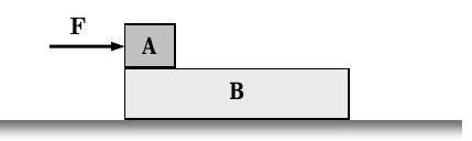
Figure \(\PageIndex{4}\): A system consisting of two blocks held together by friction.

To study the limitations of the work-energy principle, determine the rate of change of the kinetic energy of the blocks after force \(\mathbf{F}\) is applied. Compare your results using two single-particle systems and using a combined system that includes both particles.

To make use of the work-energy principle, we must first clearly identify all of the external forces acting on the system. This is done below for the System \(A B\), System \(A\), and System \(B\).

System \(AB\)

System \(A\)

System \(B\)

Figure \(\PageIndex{5}\): Free-body diagrams for systems consisting of blocks \(AB\), of block \(A\) only, and of block \(B\) only.

For system \(A\), the work-energy principle can be written as \[\begin{aligned} \frac{d}{dt} \left(E_{K}+E_{G P}\right)_{A} &= \dot{W}_{\text {mech}} \\ \frac{d E_{K, \ A}}{dt} + \underbrace{ \cancel{ \frac{d E_{GP, \ A}}{dt} }^{=0} }_{\text {No change in elevation}} &= \left(\mathbf{F} \cdot \mathbf{V}_A\right) + \underbrace{ \cancel{ \left(\mathbf{F}_{NA} \cdot \mathbf{V}_A\right) }^{=0} }_{\begin{array}{c} \text{Force and velocity} \\ \text{are perpendicular} \end{array}} + \underbrace{ \left(\mathbf{F}_f \cdot \mathbf{V}_A\right) }_{\text{Friction}} \\ \frac{dE_{K, \ A}}{dt} &= \left(F \cdot V_A\right) + \underbrace{ \left(-F_f \cdot V_A\right) }_{\begin{array}{c} \text{Friction force opposes} \\ \text{motion with velocity } V_A \end{array}} \quad \rightarrow \quad \boxed{ \frac{d}{dt} \left(m_A \frac{V_A ^{\ 2}}{2} \right) = \left( F - F_f \right) \cdot V_A } * \end{aligned} \nonumber \]

Note how for system \(B\), the work-energy principle can be written as \[\begin{aligned} \frac{d}{dt} \left(E_K + E_{GP}\right)_B &= \dot{W}_{\text{mech}} \\ \frac{d E_{K, \ B}}{dt} + \underbrace{ \cancel{\frac{d E_{GP, \ B}}{dt}}^{=0} }_{\text{No change in elevation}} &= \underbrace{ \cancel{ \left(\mathbf{F}_N \cdot \mathbf{V}_B\right) }^{=0} }_{\begin{array}{c} \text{Force and velocity} \\ \text{are perpendicular} \end{array}} + \underbrace{ \cancel{ \left(\mathbf{F}_{NA} \cdot \mathbf{V}_B\right) }^{=0} }_{\begin{array}{c} \text{Force and velocity} \\ \text{are perpendicular} \end{array}} + \underbrace{ \left(\mathbf{F}_f \cdot \mathbf{V}_B\right) }_{\text{Friction}} \\ \frac{d E_{K, \ B}}{dt} &= \left(F_f \cdot V_B\right) \quad \rightarrow \quad \boxed{ \frac{d}{dt} \left( m_B \frac{V_B ^{\ 2}}{2} \right) = \left(F_f \cdot V_B\right) } ** \end{aligned} \nonumber \]

where the velocity used in calculating the mechanical power must be the velocity of the block \(B\) based on our derivation of the work-energy principle for a particle.

Now adding these two equations together, we have \[ \begin{aligned} \left. \begin{array}{c} \dfrac{d}{dt} \left(m_{A} \dfrac{V_{A}{ }^{2}}{2}\right) = \left(F-F_{f}\right) \cdot V_{A} \\ + \\ \dfrac{d}{dt} \left(m_B \dfrac{V_{B}{ }^{2}}{2} \right) = F_f \cdot V_B \end{array} \right\} \quad \rightarrow \quad & \frac{d}{dt} \left(m_A \frac{V_{A}{ }^{2}}{2}\right) + \frac{d}{dt} \left(m_B \frac{V_{B}{ }^{2}}{2} \right) = \left(F-F_f\right) \cdot V_A + F_f \cdot V_B \\ & \boxed{ \ \underbrace{ \frac{d}{dt} \left(m_A \frac{V_{A}{ }^{2}}{2}\right) + \frac{d}{dt} \left(m_B \frac{V_{B}{ }^{2}}{2}\right) }_{\begin{array}{c} \text{Rate of change of the kinetic energy} \\ \text{of blocks } A \text{ and } B \end{array}} = F \cdot V_A - \left(F_f\right) \cdot \left(V_A - V_B\right) \ }*** \end{aligned} \nonumber \]

For System \(A B\), the only contact forces are \(\mathbf{F}_{N}\), the normal force exerted by the ground on block \(B\), and \(\mathbf{F}\), the horizontal force applied to block \(A\). Assuming it is valid to write the work energy principle for two particles as a single system, we write

\[\begin{aligned} \frac{d \left(E_{K}+E_{G P}\right)_{sys}}{dt} &= \dot{W}_{\text {mech}} \\ \frac{d}{dt} \left[ \left(E_{K}+E_{GP}\right)_{A} + \left(E_{K}+E_{GP}\right)_{B} \right] &= \left(\mathbf{F} \cdot \mathbf{V}_{A}\right) + \underbrace{ \cancel{ \left(\mathbf{F}_{B} \cdot V_{B}\right) }^{=0} }_{\begin{array}{c} \text{Force normal} \\ \text{to velocity} \end{array}} \\ \frac{d E_{K, \ A}}{dt} + \cancel{ \frac{d E_{GP, \ A}}{dt} }^{=0} + \frac{d E_{K, \ B}}{dt} + \cancel{ \frac{d E_{GP, \ B}}{dt} }^{=0} &= F \cdot V_{A} \quad \rightarrow \quad \boxed{ \frac{d}{dt} \left(m_{A} \frac{V_{A}{ }^{2}}{2}\right) + \frac{d}{dt}\left(m_{B} \frac{V_{B}{ }^{2}}{2}\right) = F \cdot V_{A} } * * * * \end{aligned} \nonumber \]

If the work-energy principle applies to systems with two particles, then Eq. \({***}\) and Eq. \(^{* * * *}\) should give us the same information. Under what conditions are these two equations identical?

Condition 1: The friction force is zero.

Condition 2: There is no relative velocity between the particles, i.e. \(V_{A}=V_{B}\). Thus it would appear that the work-energy principle accurately describes the behavior of a system with multiple particles only under a limited set of conditions.

Thus it would appear that the work-energy principle accurately describes the behavior of a system with multiple particles only under a limited set of conditions.

Fortunately, experiences like the one above allow us to establish general guidelines for the use of the work-energy principle:

The work-energy principle can be applied to any closed system if (1) the system can be modeled as a collection of particles, i.e. moment of inertia of each subsystem is negligible, and (2) there is no friction inside the system.

As we will show shortly, these limitations are related to the fact that the work-energy principle is a restricted application of the general conservation of energy principle. Now we will turn to an application of the work-energy principle:

Example — Movin' boxes

Two boxes rest on individual inclined planes and are connected by a pulley as shown in the figure. The mass of each box is \(12 \mathrm{~kg}\) and the boxes rest on frictionless surfaces. If the system is released from rest, determine the magnitude of the velocity of the weights when they have moved a distance \(L=1 \mathrm{~m}\) along the planes.

Figure \(\PageIndex{6}\): A pulley at the intersection of two inclined planes supports a string connected to boxes on each plane.

Solution

Known: Two boxes connected by a pulley and cable slide on inclined surfaces.

Find: The velocity of the boxes when they have traveled a distance of \(1 \mathrm{~m}\) along the planes.

Given: See the figure above.

Strategy \(\rightarrow\) There are at least three possible ways to attempt this problem. One is to apply conservation of linear momentum. A second is to apply conservation of angular momentum. A third is to try the work-energy principle. (This is, in reality, just an alternate way to apply conservation of linear momentum.)

System \(\rightarrow\) Both blocks, the pulley, the cable, and the pulley support.
Property to count \(\rightarrow\) Lets try mechanical energy, i.e. work-energy principle.
Time interval \(\rightarrow\) Start with the finite-time form since we have a finite displacement.

First we should sketch the free-body diagram and identify all of the external forces acting on our system. If you look carefully you will see the weights of the two boxes, the normal forces on the two boxes, two forces where we cut the pulley support, and the weight of the pulley and its support. (Look at the figure and find each of these.) You will also see the positive \(z\)-coordinate which points opposite to the direction of gravity.

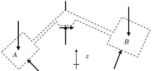
Figure \(\PageIndex{7}\): Free-body diagram of the system consisting of the boxes, their connecting cable, and the pulley the cable wraps around.

Now to apply the principle of work-energy to this system, we must model the closed system as a collection of particles with no internal friction.

\[ \begin{align*} \Delta \left(E_K + E_{GP}\right)_{sys} &= W_{\text{mech}} \\ \Delta E_K + \Delta E_{GP} &= \underbrace{ \cancel{ W_{\text{mech}} }^{=0} }_{\begin{array}{c} \mathbf{F} \cdot d\mathbf{s}=0 \text{ for all} \\ \text{contact forces} \end{array}} \\ \Delta \left(m_A \dfrac{V_{A}{ }^{2}}{2} + m_B \frac{V_{B}{ }^{2}}{2}\right) + \Delta \left(m_A gz_A + m_B gz_B\right) &= 0 \\ \underbrace{ \left(m_A \frac{V_{A}{ }^{2}}{2} + m_B \frac{V_{B}{ }^{2}}{2}\right)_2 }_{\begin{array}{c} V_A=V_B=V \text{ since connected} \\ \text{by inextensible cable} \end{array}} + \left(m_A gz_A + m_B gz_B\right)_2 &= \underbrace{ \cancel{ \left(m_A \frac{V_{A}{ }^{2}}{2} + m_B \frac{V_{B}{ }^{2}}{2}\right) }^{=0} }_{\text{Initially stationary, no velocity}} + \left(m_A gz_A + m_B gz_B\right)_1 \\[4pt] \left(m_A + m_B\right) \frac{V_{2}{ }^{2}}{2} &= m_A g \left(z_1 - z_2\right)_A + m_B g \left(z_1 - z_2\right)_B \end{align*} \nonumber \]

In developing this equation we have also assumed that there is no friction inside the system and the rotation of the pulley is insignificant, i.e. it has a negligibly small mass moment of inertia about its axis of rotation.

Carefully notice that the force of gravity, or the weight of the masses, does not do any work on the system. Including weight as a force in the work term is a common mistake and results in a double counting of the effect of gravity. Ignoring the effect of gravity in the work term is a direct consequence of our definition of mechanical work in terms of surface (contact) forces. We can handle the effect of gravity in two different ways. If we include the force of gravity in the work term, there is no gravitational potential energy. If we handle the effect of gravity through the gravitational potential energy term, then only surface forces do work. To be consistent with the general conservation of energy principle, we have elected to use the latter approach.

To go further, we must indicate how the change in elevation is related to the displacement of the boxes along the planes. Assume that box \(A\) moves up the plane and box \(B\) moves down the plane.

Therefore \[\left(z_{2}-z_{1}\right)_{A} = L \sin \theta \quad \text { and } \quad \left(z_{2}-z_{1}\right)_{B}=-L \sin \alpha \nonumber \]

Substituting this back into the result from the work-energy principle, we have \[\begin{aligned} \left(m_{A}+m_{B}\right) \frac{V_{2}{ }^{2}}{2} &= m_{A} g\left(z_{1}-z_{2}\right)_{A} + m_{B} g\left(z_{1}-z_{2}\right)_{B} \\ &= -m_{A} g\left(z_{2}-z_{1}\right)_{A} - m_{B} g\left(z_{2}-z_{1}\right)_{B} \\ &=-m_{A} g(L \sin \theta) - m_{B} g(-L \sin \alpha) \quad \text { but } \quad m_{A}=m_{B}=m_{Box} \\ \left(2 m_{box} \right) \frac{V_{2}{ }^{2}}{2} &= m_{box} g L(\sin \alpha-\sin \theta) \\[4pt] V^{2} &= g L(\sin \alpha-\sin \theta) = \left(9.81 \ \frac{\mathrm{m}}{\mathrm{s}^{2}}\right) (1 \mathrm{~m}) \left(\sin 30^{\circ}-\sin 45^{\circ}\right) = -2.032 \ \frac{\mathrm{m}^{2}}{\mathrm{~s}^{2}} \end{aligned} \nonumber \]

What happened? How can we take the square root of a negative number? Does this mean we have a complex velocity? Be very careful when you find yourself faced with taking the square root of a negative number. It almost always means that something is in error, as a complex velocity has no physical meaning in this problem.

What happened is that we guessed wrong about the original direction of motion! If we had assumed that box \(A\) moved down the plane and box \(B\) moved up the hill our equations for \(\Delta z\) in terms of \(L\) would have had opposite signs and \[\begin{aligned} \left(m_{A}+m_{B}\right) \frac{V_{2}{ }^{2}}{2} &= -m_{A} g\left(z_{2}-z_{1}\right)_{A} - m_{B} g\left(z_{2}-z_{1}\right)_{B} \\ &= -m_{A} g(-L \sin \theta)-m_{B} g(L \sin \alpha) \quad \text { but } \quad m_{A}=m_{B}=m_{Box} \\ \left(2 m_{box}\right) \frac{V_{2}{ }^{2}}{2} &= m_{box} g L(-\sin \alpha+\sin \theta) \\ V^{2} &= g L(\sin \theta-\sin \alpha) = \left(9.81 \ \frac{\mathrm{m}}{\mathrm{s}^{2}}\right) (1 \mathrm{~m}) \left(\sin 45^{\circ}-\sin 30^{\circ}\right) = 2.032 \ \frac{\mathrm{m}^{2}}{\mathrm{s}^{2}} \\ V &=1.43 \ \frac{\mathrm{m}}{\mathrm{s}} \text { where the elevation of } B \text{ increases and the elevation of } A \text{ decreases.} \end{aligned} \nonumber \]

Form an energy standpoint what this means is that the increased kinetic energy comes about from a decrease in the total gravitational potential energy of the system. The decrease in gravitational potential energy of box \(A\) equals the increase in gravitational potential energy of box \(B\) plus the increase in kinetic energy of the entire system.

Comment:

(a) To check this answer, try using one of the other methods.

(b) How would your answer change if the kinetic friction coefficient for surface \(B\) was \(0.1\)? [Ans: \(V=1.09 \mathrm{~m} / \mathrm{s}\) ]

7.1.3 The Mechanical Energy Balance

It is useful at this point to apply what we know about the accounting concept to better understand the work-energy principle. If we start with the rate form, Eq. \(\PageIndex{10}\) and rearrange it so that the derivatives are on the left-hand side, we have the following equation: \[\frac{d}{dt} \left(E_{K}+E_{G}\right) = \dot{W}_{\text {mech}} \nonumber \] Because the kinetic energy and gravitational energy are both extensive properties, we may increase our understanding of Eq. \(\PageIndex{12}\) by examining it in light of the accounting framework.

For this equation, the extensive property is the mechanical energy of the system. Because of their roots in mechanics, kinetic energy and gravitational potential energy are collectively referred to as mechanical energy. If the left-hand side of Eq. \(\PageIndex{12}\) represents the rate of change of an extensive property of the system, then the right-hand side must represent either a transport rate or generation rate. Because mechanical power is defined in terms of a force and velocity on the boundary, we will refer to mechanical power as a transport rate of mechanical energy.

In terms of mechanical energy, the rate form of the work-energy principle, Eq. \(\PageIndex{12}\), can be interpreted as follows:

The time rate of change (or accumulation) of mechanical energy of a system equals the net transport rate of mechanical energy into the system by mechanical work.

Unfortunately, there is no general physical principle that always satisfies this statement. However, if we restrict ourselves to mechanical energy and only consider those cases where there is no destruction or generation of mechanical energy, then Eq. \(\PageIndex{12}\) is the mechanical energy balance with no generation or destruction of mechanical energy.

A more general analysis would demonstrate that under most conditions, mechanical energy can only be destroyed within a system. Think about what happens when you drop a golf ball on the ground and let it bounce until it stops moving. Now assume you did this experiment in a vacuum to remove air friction. Initially, the golf ball has gravitational potential energy and no kinetic energy. When it finishes bouncing and rests on the ground it has less gravitational potential energy and no kinetic energy. Where did the initial mechanical energy go? We'll see later that it is irreversibly converted into internal energy — the energy of the motion of the atoms and molecules of the system.

Sometimes Eq. \(\PageIndex{12}\) is called the "conservation of mechanical energy" for a closed system. Please be careful if you want to think in these terms. In this course, we typically reserve the word "conservation" for a general usage — describing how the world always works. As we will demonstrate later using the general conservation of energy principle, Eq. \(\PageIndex{12}\) is restricted to an adiabatic, closed system where mechanical work is the only work mechanism to transport energy, and energy can only be stored as mechanical energy. See how many qualifiers have to be added just to get to "conservation of mechanical energy" from the general principle of conservation of energy.

7.1.4 An Additional Mechanical Energy — Spring Energy

If you think back to your physics class, you studied ideal springs. For our purposes an ideal spring is one that follows the same force-displacement curve regardless of the direction of displacement of the end of the spring, i.e. a spring with no hysteresis. One of the first things you learned is that the force required to compress or extend a spring is described by the equation: \[F_{\text {spring}}=k x \nonumber \] where \(k\) is the spring constant with units \(\mathrm{N} / \mathrm{m}\) or \(\mathrm{lbf} / \mathrm{in}\) or \(\mathrm{lbf} / \mathrm{ft}\) and \(x\) is the displacement of the end of the spring from its unloaded or free length position.

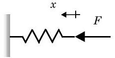
Figure \(\PageIndex{8}\): An ideal spring.

Now consider a block of mass \(m\) on a horizontal, frictionless surface as shown in Figure \(\PageIndex{9}\). Initially the block is held against the spring, and the spring is compressed to a length \(L\). The free length of the spring is \(L_{o}\). Suddenly the block is released and the block moves to the right. How could we use the mechanical energy balance to solve for the velocity of the block?

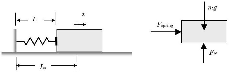
Figure \(\PageIndex{9}\): Forces acting on a block due to an expanding spring.

First we select the block as our system and draw a free body diagram showing all of the external forces acting on our system (see Figure \(\PageIndex{9}\)). Pay particular attention to the location of the \(x\)-coordinate system. Next we will assume that the block can be modeled as a particle and we can apply the finite-time form of the mechanical energy balance:

\[\begin{array}{ll} \Delta E_{K} & +\underbrace{ \cancel{ \Delta E_{G P} }^{=0} }_{\text{No change in elevation}} &= W_{\text {mech}} = \int\limits_{\mathbf{s}_{1}}^{\mathbf{s}_{2}} \mathbf{F} \cdot d \mathbf{s} = \int\limits_{x_{1}}^{x_{2}} F_{\text {spring}} \cdot dx \\ & \frac{m}{2}\left(V_{2}{ }^{2}-V_{1}{ }^{2}\right) &= \int\limits_{x_{1}}^{x_{2}} \left[k\left(L_{o}-L\right)\right] \cdot dx \quad \text { where } \quad L=L_{o}+x \\ & &= \int\limits_{x_{1}}^{x_{2}} \left[k\left(L_{o}-\left(L_{o}+x\right)\right)\right] \cdot dx \\ & &= \int_{x_{1}}^{x_{2}}[-k x] \cdot dx = -\frac{k}{2}\left(x_{2}{ }^{2}-x_{1}{ }^{2}\right) \end{array} \nonumber \]

With the initial compressed length of the spring \(L_{1}\), the velocity at any location \(x_{2}\) can be developed from the result above as follows: \[\begin{gathered} \frac{m}{2} \left(V_{2}{ }^{2}-\underbrace{V_{1}{ }^{2}}_{=0}\right) = -\frac{k}{2}\left[x_{2}{ }^{2}-x_{1}{ }^{2}\right] = -\frac{k}{2}\left[x_{2}{ }^{2}-\left(L_{1}-L_{o}\right)^{2}\right] \\ m \frac{V_{2}{ }^{2}}{2} = \frac{k}{2}\left[\left(L_{1}-L_{o}\right)^{2}-x_{2}{ }^{2}\right] \\[4pt] V_{2} = \sqrt{\frac{k}{m} \left[\left(L_{1}-L_{o}\right)^{2} - x_{2}{ }^{2}\right]} \end{gathered} \nonumber \]

Test your understanding

As a check on the result, consider what happens to the velocity of the block if \(L_{1}=L_{o}\).

What is the maximum velocity of the block and where does it occur?

What is the position of the block when the velocity goes to zero?

Now let's return to Eq. \(\PageIndex{14}\) and rearrange that result:

\[\begin{array}{l} &\frac{m}{2} \left(V_{2}{ }^{2}-V_{1}{ }^{2}\right) = -\frac{k}{2}\left(x_{2}{ }^{2}-x_{1}{ }^{2}\right) \\ &\underbrace{\frac{m}{2}\left(V_{2}{ }^{2}-V_{1}{ }^{2}\right)}_{=\Delta E_{K}} + \underbrace{\frac{k}{2}\left(x_{2}{ }^{2}-x_{1}{ }^{2}\right)}_{=\Delta E_{\text {spring}}}=0 \end{array} \nonumber \]

Notice that the term on the left-hand side only depends upon the end states of the system. This is characteristic of a property and in fact both quantities on the left-hand side are changes in extensive properties of the system. The first one is our old friend the change in kinetic energy. The second term is new and is called the change in spring (elastic) energy of the system. We define the spring (elastic) energy of the system as: \[E_{\text {spring}} \equiv \frac{1}{2} k x^{2} \nonumber \]

The ideal spring stores energy in the elastic deformation of the spring with the amount of energy directly related to the compression or expansion of the spring from its unloaded or free length.

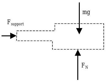
Figure \(\PageIndex{10}\): Analyzing a system with the spring inside the system.

If we treated spring energy as a form of mechanical energy and we had placed the spring inside our system (see Figure \(\PageIndex{10}\)), the mechanical energy balance with no losses would look like the following for the spring-block system: \[\Delta E_{K} + \Delta E_{G P} + \Delta E_{\text {spring}}=W_{\text {mech}} \nonumber \] To solve the problem, we would again calculate the \(W_{\text {mech}}\) for the system; however, none of the external forces contribute to the mechanical work. The normal force fails to contribute because it is perpendicular to the motion; the weight fails to contribute because it is a body force and not a surface force; and the support force holding the spring to the wall does not move. Thus the energy equation would reduce as follows:

\[\begin{array}{c} \underbrace{\Delta E_{K}}_{V_{1}=0} + \underbrace{ \cancel{\Delta E_{G P}}^{=0} }_{\text {No change in elevation}} + \Delta E_{\text {spring}} = \cancel{ W_{\text {mech}} }^{=0} \\ \Delta E_{K}+\Delta E_{\text {spring}} = 0 \\ m \frac{V_{2}^{2}}{2}+\frac{k}{2}\left(x_{2}{ }^{2}-x_{1}{ }^{2}\right)=0 \end{array} \nonumber \]

This result is identical to Eq. \(\PageIndex{14}\), the result obtained when the spring was outside the system; however, the current approach is simpler because there was no work done on the system. From a mechanical energy perspective, what is happening here is that the initial energy stored in the spring is converted to the kinetic energy of the block repeatedly as the block oscillates back and forth. This oscillation will continue forever unless there is friction internal to the system or friction between the block and the horizontal surface.

In the current section, we have extended our definition of mechanical energy to include kinetic energy, gravitational potential energy, and now spring (or elastic) energy. This by itself would be of little consequence, except we have also claimed that this new energy can be included within our existing mechanical energy balance. This experience of labeling or identifying a new form of energy and then fitting it into an existing framework is characteristic of the historical development of the conservation of energy principle. Now we will turn to this more general principle, the conservation of energy — one of the most powerful and pervasive principles of physics and engineering science.