
7.9: Thermodynamic Cycles
- Page ID
- 84366
As we study the behavior of devices, we will discover that one of the most important processes from a theoretical and a technological viewpoint is the thermodynamic cycle. More specifically we will be concerned with the performance of three types of thermodynamic cycles — power cycles, refrigeration cycles and heat pump cycles. In this section, we will discuss the basic features of a thermodynamic cycle, then we will discuss three ways to classify these devices, and finally we will consider how to measure their performance.
7.9.1 Key Features and Examples
The industrial revolution was driven in part by the development of the steam engine — a device that takes in "heat" from a fire, delivers "work" to the surroundings, and operates as a cycle. Our modern society is populated with machines and devices that either operate as a true thermodynamic cycle or can be modeled as one for purposes of analysis. The modern day internal combustion engine started out as, and is still modeled as, either an Otto cycle, a Diesel cycle, or a combined cycle. The modern-day fossil-fueled or nuclear-fueled steam power plant is modeled as a Rankine cycle. The modern gas-turbine engine, whether used in a jet engine to propel an aircraft or as part of a natural-gas-fired electrical energy peaking station, has its roots in the Brayton cycle. Some of the innovative external combustion engines currently being considered for automobiles and remote power-generation stations in remote regions are based on the Stirling cycle. One of the most famous theoretical cycles discussed in physics because of its relationship to the second law of thermodynamics is the Carnot cycle. All of these cycles are examples of power cycles.
If you are now tired of thinking of power generation but truly like to relax in your air-conditioned room, you are not finished with cycles. The guts of your window air-conditioner are modeled as a mechanical vapor-compression cycle. In fact, most refrigeration systems, whether used to cool the air in your house, maintain the food in your refrigerator, or keep those freezer display cases in the grocery cold, are also mechanical vapor-compression cycles. If you travel by air and enjoy a cool cabin you have benefited from a reversed-Brayton cycle. Sometimes you will run across a refrigerator or air conditioner that requires little or no electricity but needs a natural gas or propane flame to operate. These are examples of absorption cycles. (A company called Arkla used to manufacture these types of systems in Evansville. They were especially popular before rural electrification and are making a comeback today.) And last but not least, if your home has a heat pump, guess what? This is typically a mechanical vapor-compression cycle.
Now that you've been exposed to how much our society depends on this thing called a thermodynamic cycle, what is it? A thermodynamic cycle is a closed system that executes a series of processes that periodically return the system to its initial state.
This seems simple especially when you recognize that it is the basis for studying all of the essential devices described earlier. Since we are limited to closed systems, the rate-form of the conservation of energy equation becomes the following: \[\frac{d E_{sys}}{dt} = \dot{Q}_{\text{net, in}} + \dot{W}_{\text{net, in}} \nonumber \] which is valid at any time during the cycle. We will return to this balance shortly after we discuss the physical structure of cycles.
7.9.2 Classifying Cycles
In any discussion of thermodynamic cycles it is useful to be able to classify them. We will introduce three different ways to classify cycles — working fluids, physical structure, and purpose.
Classification by Working Fluid
If you examine the various devices mentioned earlier that operate as thermodynamic cycles, you discover that they all operate by changing the properties of a substance inside the closed system. This substance is called a working fluid. All of the examples presented earlier fall into one of two categories. In the cycles for the automobile engine or the jet engine, the working fluid remains a gas throughout the entire cycle. These are examples of cycles that operate with a single-phase working fluid. The cycles that form the basis for most refrigerators and for the fossil-fueled steam power plants change the phase of the working fluid from a liquid to a vapor and then back to a liquid in the cycle. These are examples of cycles that operate with a two-phase working fluid. These distinctions will not be very significant to us this quarter; however, to the designer they have a great significance in determining the size, weight, cost, and performance of a specific cycle.
Classification by Physical Structure
Most devices that operate as or can be modeled as a thermodynamic cycle have a physical structure that fits into one of two categories — a closed, periodic cycle or a closed-loop, steady-state cycle. These are illustrated in Figure \(\PageIndex{1}\).
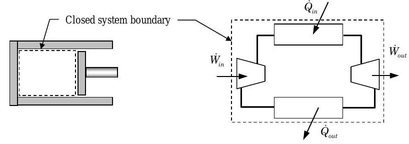
(a) Closed, periodic cycle (left) (b) Closed-loop, steady-state cycle (right)
Figure \(\PageIndex{1}\): Classification of thermodynamic cycles by physical structure
The closed, periodic cycle is modeled as a fixed quantity of matter contained inside of a simple piston cylinder device [see Figure \(\PageIndex{1}\)(a)]. This cycle is characterized by spatially uniform intensive properties that vary periodically with time. This is the classic cycle that has been studied by engineers for years. It is the model for the early steam engines and is still the model for the modern internal combustion engine where a gas is compressed and expanded within a piston engine.
The closed-loop, steady-state cycle is modeled as a collection of steady-state devices that are connected together to form a closed loop of fluid as shown in Figure \(\PageIndex{1}\)(b). The closed loop of fluid forms a closed system. Steady-state devices commonly used in these cycles are pumps, turbines, compressors, heat exchangers, and valves. This cycle is characterized by spatially-nonuniform intensive properties that depend on position in the fluid loop but do not change with time. This cycle is the model for the modern gas turbine engine, the modern steam power plant, and the modern refrigerator and air-conditioner.
To investigate what conservation of energy can tell us about these cycles, we apply the rate form of the closed system energy balance to each type of cycle and manipulate appropriately: \[\frac{d E_{sys}}{dt} = \dot{Q}_{\text{net, in}} + \dot{W}_{\text{net, in}} \nonumber \]
| \(\text{Closed-periodic cycle}\) | \(\text{Closed-loop, steady-state cycle}\) |
| \[ \begin{array}{l} \underbrace{\int\limits_{t}^{t + \Delta t_{\text{cycle}}} \left(\frac{d E_{sys}}{dt}\right) dt}_{\begin{array}{c} \text{Integrated over one period} \\ \text{of the cyle} \end{array}} = \int\limits_{t}^{t + \Delta t_{\text{cycle}}} \dot{Q}_{\text{net, in}} + \int\limits_{t}^{t + \Delta t_{\text{cycle}}} \dot{W}_{\text{net, in}} \\ \underbrace{\left. E_{sys} \right|_{t + \Delta t_{\text{cycle}}} - \left. E_{sys} \right|_{t}}_{=0. \text{ Why?}} = Q_{\text{net, in}} + W_{\text{net, in}} \\ 0 = Q_{\text{net, in}} + W_{\text{net, in}} \\ Q_{\text{net, in}} = -W_{\text{net, in}} = W_{\text{net, out}} \end{array} \nonumber \] | \[\begin{array}{l} \underbrace{ \cancel{\dfrac{d E_{sys}}{dt}}^{=0} }_{\begin{array}{c} \text{Steady-state} \\ \text{system} \end{array}} = \dot{Q}_{\text{net, in}} + \dot{W}_{\text{net, in}} \\ { } \\ 0 = \dot{Q}_{\text{net, in}} + \dot{W}_{\text{net, in}} \\ \dot{Q}_{\text{net, in}} = -W_{\text{net, in}} = W_{\text{net, out}} \end{array} \nonumber \] |
In both cycles, we discover something similar — The net heat transfer (or transfer rate) of energy into the system equals the net work transfer (or transfer rate) of energy out of the system for thermodynamic cycle.
This result leads to the common interpretation of a thermodynamic cycle as an energy conversion device for converting heat transfer of energy into work transfers of energy.
Classification by Purpose
Experience has shown that work transfers of energy are more valuable than heat transfers of energy. This means that we can do more things with a work transfer of energy than we can with a heat transfer of energy. Because of this, we will choose to define the purpose of a device in terms of the work transfer of energy for the cycle.
The claim is made that work is more valuable than heat transfer. Can you think of any system and process that can only be done by a heat transfer of energy? [If you can, could the system be redefined and the heat transfer be replaced by a work transfer of energy?]
If the net power or work out of the cycle is positive, then we call the device a power cycle or heat engine: \[\dot{W}_{\text {net, out }} \text { or }\left.W_{\text {net, out }}\right|_{\text {cycle}}>0 \quad \rightarrow \quad \text { Power cycle } \nonumber \] The purpose of a power cycle is to take a net amount of energy by heat transfer from the surroundings and transfer back to the surroundings a net amount of energy as work.
If the net power or work into the cycle is positive, then we call the device a refrigeration or heat pump cycle (sometimes this is called a reversed power cycle): \[\dot{W}_{\text {net, in }} \text { or }\left.W_{\text {net, in }}\right|_{\text {cycle }}>0 \quad \rightarrow \quad \begin{array}{c} \text { Refrigeration or } \\ \text{ heat pump cycle } \end{array} \nonumber \] The purpose of a refrigeration or heat pump cycle is to take a net amount of energy by work from the surroundings and transfer a net amount of energy by heat transfer back to the surroundings. More specifically, these cycles take in an amount of energy by heat transfer at a low temperature and reject a larger amount of energy by heat transfer at a higher temperature. A refrigeration cycle is built to maximize the amount of energy that can be transferred into the cycle by heat transfer at the low temperature. A heat pump cycle is built to maximize the amount of energy that can be transferred out of the system at the high temperature.
7.9.3 Quantifying Cycle Performance
Given a specific cycle, it is helpful to be able to quantify its performance so that we can compare it with other cycles that do the same thing. As a working engineer, you may be faced with buying a piece of equipment from one of several manufacturers or vendors. Although each vendor's product does the same task, it will undoubtedly have a different performance. So we need some way to compare performance between vendors.
Measure of Performance (MOP)
Based on our discussion of the purpose of cycles, it would seem that one way to evaluate the performance of a cycle is to compare two things: what it costs vs. the desired product or output.
Using this idea, we can define a measure of performance (MOP) for a cycle as follows: \[MOP = \frac{\text { (Desired product or output) }}{\text { (What it costs to operate the cycle) }} \nonumber \] If you think of a cycle as an energy conversion device, an equally good name for the measure of performance would be an energy conversion ratio (ECR). These terms will be used interchangeably in this course. To go further, we must examine each cycle and determine what constitutes the desired output and the cost to operate the cycle.
MOP for a Power Cycle
If you now examine a power cycle, you can identify three interactions with the surroundings: heat transfer into the system, heat transfer out of the system, and a net work transfer of energy out of the system (see Figure \(\PageIndex{2}\)). Now what is the desired output and what is the cost to operate a power cycle?
- Desired output? \(\rightarrow\) Net work transfer of energy out of the system.
- Cost? \(\rightarrow\) Heat transfer of energy into the system.
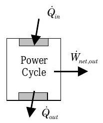
Figure \(\PageIndex{2}\): Power cycle or heat engine.
Given this information, the MOP for a power cycle is called the cycle thermal efficiency \(\eta\) and is defined as follows: \[\eta = \frac{\dot{W}_{\text {net, out}}}{\dot{Q}_{\text {in}}} \leq 1 \quad\quad \begin{array}{c} \text{ Cycle } \\ \text { Thermal Efficiency } \end{array} \nonumber \] As indicated above, the thermal efficiency can take on values between 0 and 1. The worst power cycle would be one that takes in and rejects an equal amount of energy by heat transfer and produces no power out. On the other hand, the best power cycle would appear to be one that exchanges energy by heat transfer with only a single source and turns this energy completely into a power output. (We will show in the next chapter that it is impossible to build a power cycle with a thermal efficiency of one.) Some of the best fossil-fueled steam power plants only have efficiencies of approximately \(30 \%\).
The thermal efficiency is defined in terms of the total heat transfer into the system. Would it make sense to define it in terms of the net heat transfer into the system? Why not?
MOP for a Refrigeration Cycle
If you now examine a refrigeration cycle, you can identify three interactions with the surroundings: heat transfer into the system, heat transfer out of the system, and a net work transfer of energy into the system (see Figure \(\PageIndex{3}\)). Now what is the desired output, and what is the cost to operate a refrigeration cycle?
- Desired output? \(\rightarrow\) Heat transfer of energy into the system.
- Cost? \(\rightarrow\) Net work transfer of energy into the system
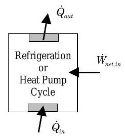
Figure \(\PageIndex{3}\): Refrigeration or heat pump cycle.
Given this information the MOP for a refrigeration cycle is called the Coefficient of Performance \(\mathrm{COP}_{\mathrm{ref}}\) and is defined as follows: \[0 \leq COP_{\text {ref}} = \frac{\dot{Q}_{\text {in }}}{\dot{W}_{\text {net, in}}} \quad\quad \begin{array}{c} \text { Coefficient of Performance } \\ \text { (Refrigeration Cycle) } \end{array} \nonumber \] As indicated above, the COP for a refrigeration cycle can take on values greater than zero. The worst refrigeration cycle would be one that takes in no energy by heat transfer. On the other hand, there appears to be no upper limit on the COP. (We will show in the next chapter that there is in fact an upper limit on the COP value for a refrigeration cycle.)
MOP for a Heat Pump
If you examine a heat pump cycle, you can identify three interactions with the surroundings: heat transfer into the system, heat transfer out of the system, and a net work transfer of energy into the system (see Figure \(\PageIndex{3}\)). Now what is the desired output, and what is the cost to operate a heat pump cycle?
- Desired output? \(\rightarrow\) Heat transfer of energy out of the system.
- Cost? \(\rightarrow\) Net work transfer of energy into the system
Given this information, the MOP for a heat pump cycle is called the Coefficient of Performance \(\text{COP}_{\text{HP}}\) and is defined as follows: \[1 \leq COP_{\mathrm{hp}} = \frac{\dot{Q}_{\text {out}}}{\dot{W}_{\text {net, in}}} \quad\quad \begin{array}{c} \text { Coefficient of Performance } \\ \text { (Heat Pump Cycle) } \end{array} \nonumber \] As indicated above the COP for a heat pump cycle can take on values greater than one. The worst heat pump cycle would be one that takes in no energy by heat transfer and converts all of the work transfer into the system into heat transfer out of the system. On the other hand, there appears to be no upper limit on the COP. (We will show in the next chapter that there is in fact an upper limit on the COP value for any heat pump cycle.)
An application of MOP's
Measures of performance are typically used in one of two ways:
- you are asked to compute the MOP for a specific cycle given all of the necessary information.
- you are given the MOP and another piece of information, e.g. refrigeration capacity (heat transfer into a refrigeration cycle), and then asked to find the other heat transfer and work transfers.
Here are examples of each type of question:
The measured performance of a power cycle indicates that the heat transfer into the cycle is \(800 \mathrm{~kJ} / \mathrm{cycle}\) and the heat transfer out of the cycle is \(600 \mathrm{~kJ} / \mathrm{cycle}\). Determine the thermal efficiency of this power cycle.
Solution
\[\left.\begin{array}{l} Q_{\text {in}} = 800 \mathrm{~kJ} / \mathrm{cycle} \\ \mathrm{Q}_{\text {out}} = 600 \mathrm{~kJ} / \mathrm{cycle} \end{array}\right\} \rightarrow \left\{ \begin{array}{c} 0=Q_{\text {in}}-Q_{\text {out}}-W_{\text {net, out}} \\ W_{\text {net, out}}=Q_{\text {in}}-Q_{\text {out}} \\ W_{\text {net, out}}=(800-600) \dfrac{\mathrm{kJ}}{\mathrm{cycle}} = 200 \dfrac{\mathrm{kJ}}{\mathrm{cycle}} \end{array}\right\} \rightarrow \eta=\frac{W_{\text {net, out}}}{Q_{\text {in}}} = \frac{(200)}{(800)} = 0.25 \nonumber \]
A heat pump is designed to deliver \(10,000 \mathrm{~Btu} / \mathrm{~h}\) of heat transfer with a COP of \(4\). What is the power required to operate this heat pump?
Solution
\[\left.\begin{array}{l} Q_{\text {out}}=10,000 \ \dfrac{\mathrm{Btu}}{\mathrm{h}} \\ COP_{HP} = \dfrac{\dot{Q}_{\text {out}}}{\dot{W}} \end{array}\right\} \quad \rightarrow \quad \dot{W}_{\text {net, in}} = \dfrac{\dot{Q}_{\text {out}}}{COP_{HP}} = \dfrac{\left(10,000 \ \dfrac{\mathrm{Btu}}{\mathrm{h}}\right)}{4} = 2,500 \ \dfrac{\mathrm{Btu}}{\mathrm{h}} \nonumber \] How would you calculate the heat transfer rate into the system?
Air is contained in a simple piston-cylinder device and executes a three-step cycle described in the table:
| State 1 | \(P_{1}=200 \mathrm{~kPa}; \quad T_{1}=27^{\circ} \mathrm{C}; \quad V_{1}=0.5 \mathrm{~m}^{3}\) |
|---|---|
| \(1 \rightarrow 2\) | Constant volume heating |
| State 2 | \(P_{2}=400 \mathrm{~kPa}\) |
| \(2 \rightarrow 3\) | Constant temperature (isothermal) expansion |
| State 3 | \(P_{3}=P_{1}\) |
| \(3 \rightarrow 1\) | Constant pressure (isobaric) compression |
Assuming that air can be treated as an ideal gas with room temperature specific heats, determine the following:
(a) the work and heat transfer per unit mass for each process, in \(\mathrm{kJ} / \mathrm{kg}\),
(b) the net work and net heat transfer per unit mass for the cycle, in \(\mathrm{kJ} / \mathrm{kg}\),
(c) whether the device is a power cycle (heat engine) or a refrigerator,
(d) calculate the appropriate Measure of Performance based on your answer to (b).
Solution
\[ \begin{array}{c} \text{Closed system: Air inside piston}; \quad \Delta KE = 0; \quad \Delta PE = 0 \\ \Rightarrow \Delta U = Q_{\text{in}} + W_{\text{in}} \\ \text{Divide by } m \text{ to get:} \quad \boxed{\Delta u = q + w} \end{array} \nonumber \]
\[ \begin{array}{c} \text{Since there is only } PdV \text{ work, } \quad W_{\text{in}} = - \int\limits_{1}^{2} P \ d V\kern-0.8em\raise0.3ex- \\ \text{Divide by } m \text{ to get:} \quad \boxed{w_{\text{in}} = - \int P \ d \upsilon} \end{array} \nonumber \]
\[ \begin{aligned} 1 \rightarrow 2: \text{ Constant Volume} \\ \Delta u &= q_{1 \text{-} 2} - \cancel{ w_{1 \text{-} 2}}^{=0} \\ w_{1 \text{-} 2} &= 0 \quad \text{ since } \upsilon = \text{a constant} \\[4pt] \text{Ideal gas model:} \quad \frac{P_2 \cancel{V\kern-0.8em\raise0.3ex-_2}}{P_1 \cancel{V\kern-0.8em\raise0.3ex-_1}} &= \frac{\cancel{m} \cancel{R} T_{2}}{\cancel{m} \cancel{R} T_{1}} \\ \Rightarrow T_{2} &= \frac{P_2}{P_1} T_{1} = (2)(600 \mathrm{~K}) = 600 \mathrm{~K} \\[4pt] q_{1 \text{-} 2} &= u_{2} - u_{1} \\ &= C_{v} \left(T_{2}-T_{1}\right) \\ &= (0.718)(600-300) \frac{\mathrm{kJ}}{\mathrm{kg}} \end{aligned} \nonumber \]
\[ \boxed{q_{1 \text{-} 2} = 215.40 \frac{\mathrm{kJ}}{\mathrm{kg}}} \nonumber \]
\[ \begin{aligned} 2 \rightarrow 3: \text{ Isothermal} \\ \Delta u &= C_{v} \cancel{\left(T_{2}-T_{1}\right)}^{=0} = 0 \\ \cancel{\Delta u}^{=0} &= q+w \\ q_{2 \text{-} 3} &= -w_{2 \text{-} 3} \\[4pt] w_{2 \text{-} 3} &= - \int\limits_{2}^{3} P \ d\upsilon \quad \text{ but } P=\frac{RT}{\upsilon} \\ w_{2 \text{-} 3} &= - \int\limits_{2}^{3} \frac{RT}{\upsilon} \ d\upsilon \\ w_{2 \text{-} 3} &= -RT_{2} \ln \left(\frac{\upsilon_{3}}{\upsilon_{2}}\right) \\[4pt] P_{3} \upsilon_{3} = P_{2} \upsilon_{2} \rightarrow \frac{\upsilon_{3}}{\upsilon_{2}} &= \frac{P_{2}}{P_{3}} \quad \text{ where } P_{3} = P_{1} \\ \Rightarrow \frac{\upsilon_{3}}{\upsilon_{2}} = \frac{P_{2}}{P_{1}} = \frac{400}{200} &= 2 \\[4pt] w_{2 \text{-} 3} &= -(0.287)(600) \ln (2) \mathrm{~kJ} / \mathrm{kg} \end{aligned} \nonumber \]
\[ \begin{array}{c} \boxed{ w_{2 \text{-} 3} = -119.36 \frac{\mathrm{kJ}}{\mathrm{kg}} } \\ \boxed{ q_{2 \text{-} 3} = 119.36 \frac{\mathrm{kJ}}{\mathrm{kg}} } \end{array} \nonumber \]
\[ \begin{aligned} 3 \rightarrow 1: \text{ Isobaric Compression} \\ \Delta u &= q+w \\ w_{3 \text{-} 1} &= - \int\limits_{3}^{1} P \ d \upsilon \\ &= - \underbrace{P_{3}}_{= P_1} \left(\upsilon_{1} - \upsilon_{3}\right) \\ &= -P_{1} \upsilon_{1} \left(1 - \frac{\upsilon_{3}}{\upsilon_{1}}\right) \\ &= -RT_{1} \left(1 - \frac{P_{2}}{P_{1}}\right) \\ \frac{\upsilon_{3}}{\upsilon_{1}} &= \frac{P_{2}}{P_{1}} \text{ since } P_{3} \upsilon_{3} = P_{2} \upsilon_{2}; \quad P_{3} = P_{1}; \quad \upsilon_{2} = \upsilon_{1} \\ &\Rightarrow P_{1} \upsilon_{3} = P_{2} \upsilon_{1} \end{aligned} \nonumber \]
\[ \begin{array}{l} { } \\ w_{3 \text{-} 1} = -(0.287)(300)(1-2) \dfrac{\mathrm{kJ}}{\mathrm{kg}} \\ \boxed{ w_{3 \text{-} 1} = 86.10 \ \frac{\mathrm{kJ}}{\mathrm{kg}} } \end{array} \nonumber \]
\[ \begin{aligned} q_{3 \text{-} 1} &= \left(u_{1}-u_{3}\right) - w_{3 \text{-} 1} \\ &= C_{v} \left(T_{1}-T_{3}\right) - w_{3 \text{-} 1} \\ &= \left(0.718 \ \frac{\mathrm{kJ}}{\mathrm{kg} \cdot \mathrm{K}}\right)(300-600) - w_{3 \text{-} 1} \\ &= (-215.40 - 86.10) \frac{\mathrm{kJ}}{\mathrm{kg}} \end{aligned} \nonumber \]
\[ \boxed{q_{3 \text{-} 1} = -301.50 \ \frac{\mathrm{kJ}}{\mathrm{kg}}} \nonumber \]
a) Summarizing these results:
| \(q_{\text{in}} \ (\mathrm{kJ}/\mathrm{kg})\) | \(w_{\text{in}} \ (\mathrm{kJ}/\mathrm{kg})\) | |
|---|---|---|
| \(1 \rightarrow 2\) | \(215.40\) | \(0\) |
| \(2 \rightarrow 3\) | \(119.36\) | \(-119.36\) |
| \(3 \rightarrow 1\) | \(-301.50\) | \(86.10\) |
| \[\mathbf{\sum} \nonumber \] | \(\mathbf{33.26}\) | \(\mathbf{-33.26}\) |
b) \(q_{\text{net, in}} + w_{\text{net, in}} = 0. \) This must happen for a cycle!
c) Type of cycle: \[ \begin{gathered} w_{\text{net, in}} = -33.26 \ \frac{\mathrm{kJ}}{\mathrm{kg}} \\ \Rightarrow w_{\text{net, out}} = 33.26 \ \frac{\mathrm{kJ}}{\mathrm{kg}} > 0 \\ \text{Power cycle} \end{gathered} \nonumber \]
d) Based on (c): \[ \begin{aligned} \eta &= \frac{w_{\text{net, out}}}{q_{\text{gross, in}}} = \frac{33.26}{215.40 + 119.36} \\ &= 0.09935 \Rightarrow 9.935 \% \end{aligned} \nonumber \] Only \(\simeq 10 %\) of energy brought in by heat transfer is converted to heat!
Comments:
1) The table is an essential feature of this analysis. It allows us to easily check our work.
2) The entire analysis is done on a per-mass basis.
3) This cycle is presented as a closed, periodic cycle. In theory, if we could build steady-state devices to perform these three processes, we could have a closed-loop, steady-state cycle.
If we reversed the direction of this cycle, i.e. \(1 \rightarrow 3 \rightarrow 2 \rightarrow 1\), then
| \(q_{\text{in}} \ (\mathrm{kJ}/\mathrm{kg})\) | \(w_{\text{in}} \ (\mathrm{kJ}/\mathrm{kg})\) | |
|---|---|---|
| \(1 \rightarrow 3\) | \(301.50\) | \(-86.10\) |
| \(3 \rightarrow 2\) | \(-119.36\) | \(119.36\) |
| \(2 \rightarrow 1\) | \(-215.40\) | \(0\) |
| \[ \mathbf{\sum} \nonumber \] | \(-33.26\) | \(33.26\) |
\[ w_{\text{net, in}} = 33.26 \ \mathrm{kJ} / \mathrm{kg} > 0 \Rightarrow \text{Refrigeration cycle} \nonumber \]
\[ \begin{aligned} COP &= \frac{q_{\text{in, gross}}}{w_{\text{net, in}}} = \frac{119.36+215.40}{33.26} \\ &= 10.06 \end{aligned} \nonumber \]