
7.5: Flow Work and Flow Power Revisited
- Page ID
- 84077
When the volume of a closed system is decreased, \(\mathrm{PdV}\)-work is done on the gas inside the system. Similarly, when mass flows into an open system, the mass inside the system is compressed by the entering mass.
As we count all the possible work mechanisms for transporting energy across a system boundary, we must pay particular attention to the work done at an open (or flow) boundary, especially the \(\mathrm{PdV}\)-work done on the mass inside the open system. The purpose of this section is to provide a more detailed development and explanation of flow work and flow power.
Earlier we defined flow work and flow power as follows:
Flow work is the \(\mathrm{PdV}\)-work (or compression work) done on the mass in an open system as a result of mass flowing into the system. (Although defined in terms of mass flowing into a system, mass flowing out of a system has a similar effect.)
Flow power is the time rate of doing flow work.
As shown previously, the concepts of flow work and flow power are important in developing a useful form of the conservation of energy equation for open systems. Only under extremely special cases will we have any interest in computing flow work or flow power.
If a function \(V(t)\) is continuous for values of \(t_{1} \leq t \leq t_{2}\) then there is a value of \(V\) such that \[\int\limits_{t_{1}}^{t_{2}} V(t) \ dt = V\left(t^{*}\right)\left[t_{2}-t_{1}\right] \nonumber \] where \(t_{1} \leq t^{*} \leq t_{2}\)
.png?revision=1)
Figure \(\PageIndex{1}\): Mean Value Theorem.
Systems with mass flow in
Consider a rigid tank with one inlet as shown in Figure \(\PageIndex{2}\). The interior of the tank is an open system with a constant volume (see volume inside the dashed lines). Figure \(\PageIndex{2}\) shows three snapshots of a closed system (the "gray" substance) flowing into the tank. Imagine that the closed system is the mass that has been dyed "gray." At time \(t_{1}\), the closed system is partially outside the tank [see Figure \(\PageIndex{2a}\)]. A short time later at time \(t_{2}\), the closed system occupies the same volume as the open system [see Figure \(\PageIndex{2b}\)]. Still later at time \(t_{3}\), the closed system occupies less volume than the open system [see Figure \(\PageIndex{2c}\)].
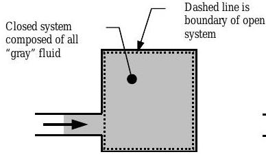 a) Closed system moving into the open system at \(t_{1} = t^* - \Delta t/2\)
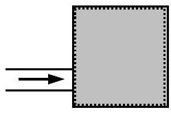.jpg?revision=1) b) Closed system coincides with open system at \(t_{2} = t^*\)
b) Closed system coincides with open system at \(t_{2} = t^*\).jpg?revision=1) c) Closed system has moved inside open system at \(t_{3} = t^* + \Delta t/2\)
c) Closed system has moved inside open system at \(t_{3} = t^* + \Delta t/2\)The compression \((\mathrm{PdV})\) work done on the mass inside the closed system during the time interval \(t_{1}\) to \(t_{3}\) is calculated using the basic equation for \(PdV\) work: \[W_{\text{in, } 1\text{-}3} = -\int\limits_{V\kern-0.5em\raise0.3ex-_{1}}^{ V\kern-0.5em\raise0.3ex-_{3}} P \ d V\kern-0.8em\raise0.3ex- \nonumber \] where \(P\) is the pressure at the moving boundary of the closed system. Using the mean value theorem from calculus, we can rewrite Eq. \(\PageIndex{2}\) as \[W_{\text {in, } 1 \text{-} 3} = -\int\limits_{V\kern-0.5em\raise0.3ex-_{1}}^{V\kern-0.5em\raise0.3ex-_{3}} P \ d V\kern-1.0em\raise0.3ex- = -\tilde{P}\left(V\kern-1.0em\raise0.3ex-_{3} - V\kern-1.0em\raise0.3ex-_{1}\right) \nonumber \] where \(P\) is a function of the closed system volume \(V\kern-0.8em\raise0.3ex-_{3}\), \(\tilde{P}=P \left(V\kern-1.0em\raise0.3ex-\right)\) and \(V\kern-1.0em\raise0.3ex-_{1} \leq \tilde{V\kern-0.8em\raise0.3ex-} \leq V\kern-0.8em\raise0.3ex-_{3}\).
The change in the volume of the closed system can be described in terms of the volumetric flow rate into the control volume as \[V\kern-1.0em\raise0.3ex-_{3} - V\kern-1.0em\raise0.3ex-_{1} = -\int\limits_{t_{1}}^{t_{3}} \dot{V\kern-0.8em\raise0.3ex-}_{\text {in}} \ dt = -\tilde{\dot{V\kern-0.8em\raise0.3ex-}}\left(t_{3}-t_{1}\right) \nonumber \] where \(\tilde{\dot{V\kern-0.8em\raise0.3ex-}}_{\text {in}} = \dot{V\kern-0.8em\raise0.3ex-}(\tilde{t})\) and \(t_{1} \leq \tilde{t} \leq t_{3}\).
Substituting Eq. \(\PageIndex{3}\) back into Eq. \(\PageIndex{2}\) gives an expression for the work done on the closed system as it moves into the tank: \[W_{\text {in, } 1 \text{-}3} = -\tilde{P}\left(V\kern-1.0em\raise0.3ex-_{3} - V\kern-1.0em\raise0.3ex-_{1}\right) = -\tilde{P}\left[-\tilde{\dot{V\kern-0.8em\raise0.3ex-}}_{\text {in}} \left(t_{3}-t_{1}\right)\right] = \tilde{P} \tilde{\dot{V\kern-0.8em\raise0.3ex-}}_{\text {in}} \left(t_{3}-t_{1}\right) \nonumber \] where \(\tilde{P}\) and \(\tilde{\dot{V}}\) are evaluated at \(\tilde{t}\) and \(t_{1} \leq \tilde{t} \leq t_{3}\).
The average work per unit time (average power) over the time interval \(t_{1}\) to \(t_{3}\) can now be written by rearranging Eq. \(\PageIndex{4}\) as follows: \[\frac{W_{\text{in, } 1 \text{-} 3}}{t_{3}-t_{1}} = \frac{W_{\text{in, } 1 \text{-} 3}}{\Delta t} = \tilde{P} \tilde{\dot{V\kern-0.8em\raise0.3ex-}}_{\mathrm{in}} \nonumber \] where \(t_{3}-t_{1}=\left(t^{*}+\Delta t / 2\right)-\left(t^{*}-\Delta t / 2\right)=\Delta t\).
The instantaneous power, as opposed to the average power, is found by taking the limit of Eq. \(\PageIndex{5}\) as \(\Delta t \rightarrow 0\) gives \[\dot{W}_{\text {flow, in}} = \displaystyle \lim_{\Delta t \rightarrow 0} \frac{W_{\text {in }, 1 \text{-} 3}}{\Delta t} = \lim_{\Delta t \rightarrow 0} \tilde{P} \tilde{\dot{V\kern-0.8em\raise0.3ex-}}_{\text {in}} = P \dot{V\kern-0.8em\raise0.3ex-}_{\text {in}} \nonumber \] \[ \begin{aligned} \text{where} \quad & \dot{W}_{\text {in, flow}}= \text{the rate of energy transferred by flow work (flow power) into the closed system that occupies the open system at time } t. \\ & P= \text{the pressure at the boundary where the mass flows into the open system at time } t. \\ & \dot{V\kern-0.8em\raise0.3ex-}_{\text {in}}= \text{the volumetric flow rate at the flow boundary at time } t. \end{aligned} \nonumber \]
Although Eq. \(\PageIndex{6}\) is correct, it is standard practice to write the flow power (rate of doing flow work) in terms of the mass flow rate. Recall that the mass flow rate is the product of the density and the volumetric flow rate. Using this result Eq. \(\PageIndex{6}\) can be rewritten as follows: \[\dot{W}_{\text {flow, in}} = P \dot{V\kern-0.8em\raise0.3ex-}_{\text {in}} = P\left(\frac{\dot{m}_{\text {in}}}{\rho}\right) = \dot{m}_{\text {in}}\left(\frac{P}{\rho}\right) \nonumber \] \[ \begin{aligned} \text{where} \quad & \dot{m}_{\text {in}}= \text{the mass flow rate at the inlet. } [\mathrm{kg} / \mathrm{s} \text{ and } \mathrm{lbm} / \mathrm{s}] \\ & \rho= \text{the density of the substance at the inlet. } [\mathrm{kg} / \mathrm{m}^{3} \text{ and } \mathrm{lbm} / \mathrm{ft}^{3}] \\ & P= \text{the pressure at the inlet. } \left[\mathrm{N} / \mathrm{m}^{2}, \mathrm{kPa}\right., \text{ bar, and } \left.\mathrm{lbf} / \mathrm{ft}^{2}\right] \end{aligned} \nonumber \]
One final change of variable is traditionally made by substituting the specific volume \(\upsilon\) for the density \(\rho\) : \[\upsilon=\frac{1}{\rho} \nonumber \] where specific volume has units of \(\mathrm{m}^{3} / \mathrm{kg}\) or \(\mathrm{ft}^{3} / \mathrm{lbm}\). Making this substitution, we obtain the traditional form for flow power: \[\dot{W}_{\text {flow, in}}=\dot{m}_{\text {in }} P \upsilon \nonumber \] Flow power has the dimensions of \([\text{Energy}]/[\text{Time}]\).
Systems with mass flow out
Using an analogous development to the one done for open systems with mass flowing in, we can show that \[\dot{W}_{\text {flow,out }}=\dot{m}_{\text {out }} P v \nonumber \]
Systems with multiple inlets and outlets
A generic open system is shown in Figure \(\PageIndex{3}\). The rate of energy transfer into the system by flow work (flow power in) is \[\dot{W}_{\text {flow, net in}} = \sum_{\text {inlets}} \dot{m}_{i}(P \upsilon)_{i}-\sum_{\text {outlets}} \dot{m}_{e}(P \upsilon)_{e} \nonumber \] Note that the flow power for a closed system is zero since the flow rates are identically zero.
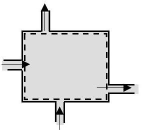
Figure \(\PageIndex{3}\): Open system with multiple inlets and outlets.