14.4.6: Coordinate Systems

Cartesian Coordinate System

While the rectangular (also called Cartesian) coordinate system is the most common, certain problems are easier to analyze in alternate coordinate systems. A coordinate system is a scheme that allows us to identify any point in the plane or in three-dimensional space by a set of numbers. In rectangular coordinates these numbers are interpreted, roughly speaking, as the lengths of the sides of a rectangular "box.''

List of some other Coordinate Systems

The choice of a coordinate system depends on the shapes that are involved in the problem at hand. There are many coordinate systems¹ including the Cartesian coordinate system, the cylindrical coordinate system, the spherical coordinate system, the ellipsoidal coordinate system, the prolate spheroidal coordinate system, and the oblate spheroidal coordinate system. In addition thee are coordinate systems that rather than focusing on shape are adapted to the subject. Examples of coordinate systems of this type are astronomical coordinate systems (based off spherical coordinate system), canonical coordinate system (mechanics: phase space), and Schwarzschild coordinate systems (relativistic: akin to a modified spherical coordinate system).

Cylindrical Coordinate System

Here we will only discuss the main coordinate system the Cartesian coordinate system (which you already know), the cylindrical coordinate system, and the spherical coordinate system. First we start with the "2D cylindrical coordinate system" we call polar coordinates.

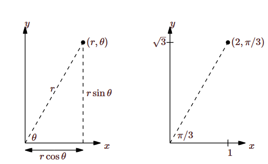
In two dimensions you may already be familiar with polar coordinates. In this system, each point in the plane is identified by a pair of numbers \((r,\theta)\). The number \(\theta\) measures the angle between the positive \(x\)-axis and a vector with tail at the origin and head at the point, as shown in Figure \(\PageIndex{1}\); the number \(r\) measures the distance from the origin to the point. Either of these may be negative; a negative \(\theta\) indicates the angle is measured clockwise from the positive \(x\)-axis instead of counter-clockwise, and a negative \(r\) indicates the point at distance \(|r|\) in the opposite of the direction given by \(\theta\). Figure \(\PageIndex{1}\) also shows the point with rectangular coordinates \( (1,\sqrt3)\) and polar coordinates \((2,\pi/3)\), 2 units from the origin and \(\pi/3\) radians from the positive \(x\)-axis.

Figure \(\PageIndex{1}\): Polar coordinates: the general case and the point with rectangular coordinates \( (1,\sqrt3)\).

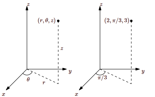
We can extend polar coordinates to three dimensions simply by adding a \(z\) coordinate; this is called cylindrical coordinates. Each point in three-dimensional space is represented by three coordinates \((r,\theta,z)\) in the obvious way: this point is \(z\) units above or below the point \((r,\theta)\) in the \(x\)-\(y\) plane, as shown in Figure \(\PageIndex{5}\). The point with rectangular coordinates \( (1,\sqrt3, 3)\) and cylindrical coordinates \((2,\pi/3,3)\) is also indicated in Figure \(\PageIndex{2}\).

Figure \(\PageIndex{2}\): Cylindrical coordinates: the general case and the point with rectangular coordinates \( (1,\sqrt3, 3)\).

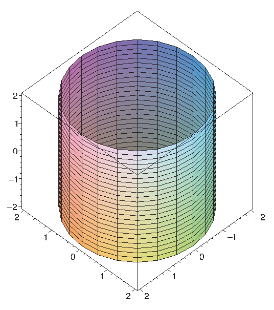
Some figures with relatively complicated equations in rectangular coordinates will be represented by simpler equations in cylindrical coordinates. For example, the cylinder in Figure \(\PageIndex{3}\) has equation \( x^2+y^2=4\) in rectangular coordinates, but equation \(r=2\) in cylindrical coordinates.

Figure \(\PageIndex{3}\): The cylinder \(r=2\).

Given a point \((r,\theta)\) in polar coordinates, it is easy to see (Figure \(\PageIndex{1}\)) that the rectangular coordinates of the same point are \((r\cos\theta,r\sin\theta)\), and so the point \((r,\theta,z)\) in cylindrical coordinates is \((r\cos\theta,r\sin\theta,z)\) in rectangular coordinates. This means it is usually easy to convert any equation from rectangular to cylindrical coordinates: simply substitute

\[\eqalign{ x&=r\cos\theta\cr y&=r\sin\theta\cr} \]

and leave \(z\) alone. For example, starting with \( x^2+y^2=4\) and substituting \(x=r\cos\theta\), \(y=r\sin\theta\) gives

\[\eqalign{ r^2\cos^2\theta+r^2\sin^2\theta&=4\cr r^2(\cos^2\theta+\sin^2\theta)&=4\cr r^2&=4\cr r&=2.\cr }\]

Of course, it's easy to see directly that this defines a cylinder as mentioned above.

Let's try this with octave as a quick script example of generating what is above.

[rflux,thetaflux] = meshgrid(linspace(0,0.7,30),linspace(0,2*pi,30));
flux = abs(2-sqrt(2)*rflux);
[r,theta] = meshgrid(2.*ones(1,30),linspace(0,2*pi,30));
surf(r.*cos(theta),r.*sin(theta),flux);

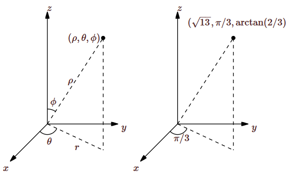
Cylindrical coordinates are an obvious extension of polar coordinates to three dimensions, but the use of the \(z\) coordinate means they are not as closely analogous to polar coordinates as another standard coordinate system. In polar coordinates, we identify a point by a direction and distance from the origin; in three dimensions we can do the same thing, in a variety of ways. The question is: how do we represent a direction? One way is to give the angle of rotation, \(\theta\), from the positive \(x\) axis, just as in cylindrical coordinates, and also an angle of rotation, \(\phi\), from the positive \(z\) axis.

Spherical Coordinate System

Roughly speaking, \(\theta\) is like longitude and \(\phi\) is like latitude. (Earth longitude is measured as a positive or negative angle from the prime meridian, and is always between 0 and 180 degrees, east or west; \(\theta\) can be any positive or negative angle, and we use radians except in informal circumstances. Earth latitude is measured north or south from the equator; \(\phi\) is measured from the north pole down.) This system is called spherical coordinates; the coordinates are listed in the order \((\rho,\theta,\phi)\), where \(\rho\) is the distance from the origin, and like \(r\) in cylindrical coordinates it may be negative. The general case and an example are pictured in Figure \(\PageIndex{4}\); the length marked \(r\) is the \(r\) of cylindrical coordinates.

Figure \(\PageIndex{4}\): Spherical coordinates: the general case and the point with rectangular coordinates \( (1,\sqrt3 , 3)\).Example \(\PageIndex{1}\)

As the cylinder had a simple equation in cylindrical coordinates, so does the sphere in spherical coordinates: \(\rho=2\) is the sphere of radius 2.

Solution

If we start with the Cartesian equation of the sphere and substitute, we get the spherical equation:

\[\begin{align*} x^2+y^2+z^2&=2^2\cr \rho^2\sin^2\phi\cos^2\theta+ \rho^2\sin^2\phi\sin^2\theta+\rho^2\cos^2\phi&=2^2\cr \rho^2\sin^2\phi(\cos^2\theta+\sin^2\theta)+\rho^2\cos^2\phi&=2^2\cr \rho^2\sin^2\phi+\rho^2\cos^2\phi&=2^2\cr \rho^2(\sin^2\phi+\cos^2\phi)&=2^2\cr \rho^2&=2^2\cr \rho&=2\cr \end{align*}\]

Example \(\PageIndex{2}\)

Find an equation for the cylinder \( x^2+y^2=4\) in spherical coordinates.

Solution

Proceeding as in the previous example:

\[\begin{align*} x^2+y^2&=4\cr \rho^2\sin^2\phi\cos^2\theta+ \rho^2\sin^2\phi\sin^2\theta&=4\cr \rho^2\sin^2\phi(\cos^2\theta+\sin^2\theta)&=4\cr \rho^2\sin^2\phi&=4\cr \rho\sin\phi&=2\cr \rho&={2\over\sin\phi}\cr \end{align*}\]

¬ So as an engineer when would you likely use the cylindrical coordinate system?

Since the cylindrical coordinate system would be best for cylindrical type objects, you would use this coordinate system for pipes (since in general pipes are cylindrical) and wires (electrical engineering). These two types of objects are ubiquitous in our society. Note you do not have to use a cylindrical coordinate system, it is just a matter of convenience. You can use any coordinate system you want. Of course it might make your problem unnecessarily difficult.

 

¬ So as a scientist when would you likely use a spherical coordinate system?

Since a spherical coordinate system would be best for spherical type objects it would be best to use this system for astronomy as the sky is replete with spherical objects (or close to spherical objects - you might want to use one of the slightly modified spherical coordinate systems for really detailed studies). Note engineers might use a spherical coordinate system for any ball like object, say ball bearings. Of course the use of said system is only to make problems easier. You can always use whatever coordinate system you want. Just be sure to be consistent.

 

How about a program to make a sphere using spherical coordinate ideas? Let us try it, eh?

[theta,phi] = meshgrid(linspace(0,pi,30),linspace(0,2*pi,30));
r = 2.*ones(1,30);
surf(r.*cos(phi).*sin(theta),r.*sin(phi).*sin(theta),r.*cos(theta));

Interestingly this looks more prolate then spherical but keep on eye on the actual scales which is 2 to -2. If you run this in your own copy of octave there will be controls for you to rotate the image.

Let us really go all out and try a prolate sphere. This is beyond the discussion but it is interesting as a program example.

[nu,phi] = meshgrid(linspace(0,pi,30),linspace(0,2*pi,30));
a = 1.*ones(1,30);
mu = 0.4*ones(1,30);
surf(a.*sinh(mu).*cos(phi).*sin(nu),a.*sinh(mu).*sin(phi).*sin(nu),a.*cosh(mu).*cos(nu));
axis([-1.2 1.2 -1.2 1.2 -1.2 1.2]);

This is probably over exaggerated but it gives you a sense of a prolate sphere. The Earth is a oblate sphere, why don't you try using the code here to help you. Use actual data to make your image realistic.

That is enough for this subject in this book/course, let us move on to the next section.

Contributors

• Template:Guichard
• Template:ContribMarshall
• Additional material and changes with a minor amount of deletions to fit with the changes. Scott Johnson, Scott Sinex, and Joshua Halpern

---

¹Here we focus on the 3D coordinate systems with some mention of 2D coordinate systems. A full explanation will also include 1D coordinate systems, etc.