14.6: Calculus

Small Pebble

Calculus (derived from Latin meaning "small pebble" {calx - limestone, chalk, small stone}) is a method of calculating with small stones which in modern times translates into a method of computation with specific rules. An interesting note is that calculus as a small stone (like kidney stones) is still used in medicine today. So why is a pebble the origin of the basis of our modern mathematical technique? Because small pebbles were used for accounting on a counting board (abacus - Latin) in ancient Rome. The origin of these counting boards are not fully known but the language is from ancient Rome/Greek/Phoenician. It is known that ancient Egyptians had counting boards but some believe it is older still.

Historically calculus is the wrong word as the calculus (infinitesimal to be precise) of today derives from geometry not calculus (simple math), but it was the formal name given by Leibniz and it stuck. For completeness sake there are many types of calculus in mathematics including infinitesimal calculus, predictive calculus, calculus of finite differences, event calculus (computer science), \(\pi\)-calculus (computer science), µ-calculus (computer science), λ-calculus(computer science), etc. Here most of the types of calculus are more reflective of the method of calculating definition.

In engineering we normally view calculus as infinitesimal calculus which includes differential calculus, integral calculus, fractional calculus, calculus of variations, and tensor calculus (see vector discussion). In the sections following we will only concern ourselves with integral and differential calculus as they are appropriate for undergraduate engineering. When we refer to calculus from here on, we will be referring to the aforementioned calculus.

Calculus was independently developed by Isaac Newton and Gottfried Leibniz (they used different methods that assure us that their work was independent). It should be noted that early cultures (ancient Egypt, ancient Greece, and ancient Chinese) used versions of something close to calculus in arcs, circles, and various other attempts to do a form of integral calculus. All of these attempts however were more akin to numerical methods¹ rather than the formal differential calculus of Newton and Leibniz. The method of exhaustion (normally credit to ancient Greece, however started in a rudimentary fashion ancient Egypt) is a famous example of "pre-calculus" that leads to limits, differentials, and area calculations (integral-like) however this method is closer to numerical methods then calculus and does not connect the differential to integral calculus. Still it was a step towards calculus.

Calculus

So to continue the theme of step-by-step development (in previous chapters), Newton's and Leibniz's calculus depended on the ancient Egyptians, the ancient Greeks, and a number of other people including Isaac Barrow (Newton's mentor), John Wallis, and Pierre de Fermat. Like other great achievements described in this course, Newton's and Leibniz's amazing achievements were build on the foundations of many mathematicians, scientists, and engineers. To be sure, Newton and Leibniz did reach the final step to have true calculus, but it was not in complete isolation².

Leibniz's work was more mathematical and theoretical (which lead to some interesting ideas that were akin to Einstein's viewpoint on space and time) where as Newton's work was more for practical purposes. For that reason we will focus on Newton's calculus (except we will still stick to Leibniz's symbols which are the symbols of our present day calculus) because it fits more with engineering philosophy.

Newton was concerned with practical issues with motion, in particular planetary motion, as non-calculus methods did not work well. Small little errors are introduced when using a numerical methods type of calculation that build-up with each successive iteration which accumulate because of propagation error. When dealing with acceleration and velocity in planetary motion this error will lead to problematic results, hence the need for a true calculus.

Infinitesimal

Calculus depends on the idea of an "infinitesimal." There is no precise definition of an infinitesimal but symbols that evoke the idea of an infinitesimal are \(\epsilon\),\(\delta\), and dt. The first two symbols are usually used in mathematical analysis (or sometimes engineering numerical methods class) and the last symbol is the one used in your engineering, science, calculus classes and herein.

The idea of the infinitesimal is really just the idea of incredibly small which we express either as \(dt = \lim_{\Delta t \to 0} \Delta t\) or \(dt = \lim_{\Delta t \to \infty} \frac{1}{\Delta t} \). Again this is more an idea not a rigorous precise definition because there is no way to precisely say what is "small." Here we see an aspect of art creeping into mathematics where we have a representation of something we can't precisely express.

Derivative

Total derivative

So let's go to the "definition" of the derivative (total derivative in this case). Basically it is just the tangent of a point as defined by successively reducing the rise over run (slope). The slope in the example presented here would be the average velocity but if we reduce it to a derivative it would be the instantaneous velocity. So the limit of differences on a curve goes to a differential³ form that define our instantaneous velocity.

\[v = \frac{dx}{dt} = \lim_{\Delta t \to 0} \frac{\Delta x}{\Delta t}\]

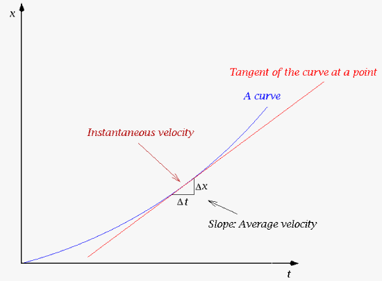A depiction of the idea of a derivative with the tangent of a curve at a point being the instantaneous velocity or the derivative of x over time.

Partial Derivative

What about a function with two variables or more variables? In this case we need to move to partial derivatives. So if we have a function, f(x,y) then the differential of the function is a combination of partial derivatives.

\[df(x,y) = \frac{\partial{f}}{\partial{x}}dx + \frac{\partial{f}}{\partial{y}}dy\]

It is easy to see that if we suddenly remove the dependency on y and just have f(x) then the above equation reduces to \(\frac{df}{dx}=\frac{\partial{f}}{\partial{x}}\). A partial derivative acts differently then a total derivative only if our function is dependent on two or more variables. Also, if our function is dependent on two or more variable then you must use partial derivatives. In the above example the x position only depends on time so \(v = \frac{dx}{dt}\) is correct. But if we had a function that depends on time and position like velocity is in some formalisms in fluid dynamics then we would need a partial derivative to define acceleration \(a = \frac{\partial{v}}{\partial{t}}\) with some other components that we will leave for later classes in your future.

Integral

Riemann sum

Integrals⁴ can be "defined" in a similar way to derivatives at least if we are finding an area or something similar.

\[F(x) = \int_a^b {f(x)dx} = \lim_{||\Delta x|| \to 0} \sum_{i=1}^n f(x_i) {\Delta x}\]

or in a manner more fitting for numerical methods.

\[ F =\sum_{i=1}^n f(x_i) (x_i - x_{i-1})\]

There are many versions of this depending how you wish to define the \(\Delta x\) which could be \(x_{i+1}-x_i\), \(\frac{x_i - x_{i-1}}{2}\), etc. In numerical methods to improve accuracy this usually gets even more complex. This is one of the reasons a numerical methods class or section of a class (say in Signals and Systems) is needed for a full understanding of engineering and science.

Quadrature

The other idea is integration or quadrature which is the idea of finding the exact area of objects. As an example the area of a circle depends on its radius, R and is best done in polar coordinates, r and \(\theta\).

\[A = \int_{0}^{2\pi}\int_{0}^{R} r dr d\theta\]

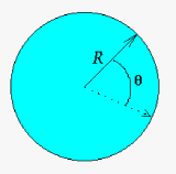With integration we can get the exact area of a circle by integrating from through each "infinitesimal" section of \(\theta\) over the \(2\pi\) circumference while integrating from the center of the circle to the outer edge.

\[A = \theta \vert_0^{2\pi} \int_{0}^{R} r dr\]

\[A = 2\pi \int_{0}^{R} r dr\]

\[A = 2\pi \frac{1}{2} r^2 \vert_0^R\]

\[A = \pi R^2\]

The following theorems define calculus in a formal sense. While you might see these as not useful in your engineering applications, they are important in building essential concepts in numerical methods.

Fundamental Theorems of Calculus

• If f(x) is continuous on a closed interval [a,b] and if F is the anti-derivative we have the an integral.

\[\int_a^b f(t) dt = F(b) - F(a)\]

• If f(x) is continuous on the open interval (a,b) then at any point \(\theta\), F can be defined as an integral of the function f.

\[F(x) = \int_{\theta}^x f(\tau) d\tau\]

\[F'(x) = f(x)\]

Mean-Value Theorem

• If f(x) id differentiable on the open interval (a,b) and continuous on the closed interval [a,b], then there must exist at least one point, say \(\theta\) in (a,b) such that

\[f'(\theta) = \frac{f(b)-f(a)}{b-a}\]

From these theorems we can make some other statements (equations) that are useful. For the anti-derivative we have an equation that represents a mean value as \(F(b)-F(a) = F'(\theta)(b-a)\). For an estimate of the integral of the function f(x) we have \(\int_a^b f(\tau) d\tau = f(\theta)(b-a)\) where \(\theta\) is an average value of f(t) on [a,b]. And for the integral of a function that can be factored into the function f(x) and another function, say g(x), we can say \(\int_a^b f(\tau)g(\tau)d\tau = f(\theta) \int_a^b g(\tau) d\tau\) where \(f(\theta)\) is a g(t)-weighted average of f(t) on [a,b].

The theorems help to establish the theory of calculus which you will learn in your calculus classes. From here we will go on to the sections that will detail some practical applications of this (as is suitable for a introduction class).

---

¹Numerical methods (see parachute person) are a computational method that approximates more rigorous but intractable mathematical equations. This leads to a fun fact relating to ancient Egypt: Ancient Egyptian mathematics were a form of binary mathematics (just like how electronic computers work) and practical calculus on computers in the present are accomplished by numerical methods. Note the numerical methods in the present are somewhat different from numerical methods of the past in that the theories of calculus and the electronic computers have modified the methods (to improve them).

²While the beginning of Newton's fluxions (his term for calculus) was build on others work he did actually finished up his theories in isolation from the plague (just like people isolated themselves from the COVID pandemic). The fluxion is what we now call a time derivative. The time derivative symbol is the only symbol of Newton's method that is still in use.

³A quick note on notation. Derivatives can be expressed with certain "short-cut" symbols (the apostrophe and the dot):

\[f'(x) = \frac{df(x)}{dx}\]

\[\dot{f(t)} = \frac{df(t)}{dt}\]

Here note that the apostrophe is for derivatives not time-based, where as the dot is used for time derivatives only. The dot derivative is the only symbol of Newton's that is still used today.

⁴It should be noted that there are many types of integrals. Here we are just discussing the basic integral you learn when you first start calculus. Other types of integrals are line integral (scalar fields and vector fields), contour integral (complex plane), surface integral (scalar fields and vector fields), volume integral, path integral (arcs), etc. The path integral has multiple definitions of which one is the line integral. The definitions the at least one of the authors use distinguishes line integral for path integral. See Wolfram's Mathworld for details. These integrals will be in later classes after you finish your freshman calculus and sophomore differential equations.