14.2.7.6: The Laplace Transform

The causal version of the Fourier transform is the Laplace transform; the integral over time includes only positive values and hence only deals with causal impulse response functions¹. In our discussion, the Laplace transform is chiefly used in control system analysis and design.

Definition of Laplace Transform

The Laplace transform projects time-domain signals into a complex frequency-domain equivalent. The signal \(y(t)\) has transform \(Y (s)\) defined as follows:

\[ Y(s) = L(y(t)) = \int\limits_{0}^{\infty} y(\tau) e^{-s \tau} \, d\tau ,\]

where \(s\) is a complex variable, properly constrained within a region so that the integral converges. \(Y(s)\) is a complex function as a result. Note that the Laplace transform is linear, and so it is distributive: \(L(x(t) + y(t)) = L(x(t)) + L(y(t))\). The following tables give a list of some useful transform pairs and other properties, for reference.

Table of Laplace Transforms

Table \(\PageIndex{1}\): List of some common Laplace transforms. Contributors: Wikipedia.

Function	Time domain \(f(t) = \mathcal{L}^{-1} \{F(s)\} \)	Laplace s-domain \(F(s) \mathcal{L} \{f(t)\} \)	Region of convergence
unit impulse	\(\delta(t)\)	1	all \(s\)
delayed impulse	\(\delta (t-\tau)\)	\(e^{-\tau s}\)	Re\((s) > 0\)
unit step	\(u(t)\)	\(\dfrac{1}{s}\)	Re\((s) > 0\)
delayed unit step	\(u(t-\tau)\)	\(\dfrac {1}{s} e^{-\tau s} \)	Re\((s) > 0\)
ramp	\(t \cdot u(t)\)	\(\dfrac {1}{s^2}\)	Re\((s) > 0\)
\(n\)th power (for integer \(n\)	\(t^n \cdot u(t)\)	\( \dfrac{n!}{s^{n+1}} \)	Re\((s) > 0\) \((n > −1)\)
\(q\)th power (for complex \(q\))	\(t^q \cdot u(t)\)	\(\dfrac{\Gamma (q+1)}{s^{q+1}}\)	Re\((s) > 0\) Re\((q) > −1\)
\(n\)th root	\(\sqrt[n]{t} \cdot u(t)\)	\( \dfrac{1}{s^{\frac{1}{n} +1}} \Gamma \left( \dfrac{1}{n} +1 \right) \)	Re\((s) > 0\)
\(n\)th power with frequency shift	\(t^n e^{-\alpha t} \cdot u(t)\)	\(\dfrac{n!}{(s+\alpha)^{n+1}}\)	Re\((s) > −\alpha\)
delayed \(n\)th power with frequency shift	\((t-\tau)^n e^{-\alpha (t-\tau)} \cdot u(t-\tau)\)	\(\dfrac {n!\cdot e^{-\tau s}} {(s+\alpha)^{n+1}}\)	Re\((s) > −\alpha\)
exponential decay	\(e^{-\alpha t} \cdot u(t)\)	\(\dfrac{1}{s+\alpha}\)	Re\((s) > −\alpha\)
two-sided exponential decay (only for bilateral transform)	\(e^{-\alpha |t|}\)	\(\dfrac{2\alpha}{\alpha^2 - s^{2}}\)	\(-\alpha\) < Re\((s) < \alpha\)
exponential approach	\( (1-e^{-\alpha t}) \cdot u(t) \)	\(\dfrac{\alpha}{s(s+\alpha)}\)	Re\((s) > 0\)
sine	\(\sin(\omega t) \cdot u(t)\)	\(\dfrac{\omega}{s^2+\omega^2}\)	Re\((s) > 0\)
cosine	\(\cos(\omega t) \cdot u(t)\)	\(\dfrac{s}{s^2+\omega ^2}\)	Re\((s) > 0\)
hyperbolic sine	\(\sinh(\alpha t) \cdot u(t)\)	\(\dfrac{\alpha}{s^2-\alpha^2}\)	Re\((s) > |\alpha|\)
hyperbolic cosine	\(\cosh(\alpha t) \cdot u(t)\)	\(\dfrac{s}{s^2-\alpha^2}\)	Re\((s) > |\alpha|\)
exponentially decaying sine wave	\(e^{-\alpha t} \sin(\omega t) \cdot u(t)\)	\(\dfrac{\omega}{(s+\alpha )^2+\omega ^2}\)	Re\((s) > -\alpha\)
exponentially decaying cosine wave	\(e^{-\alpha t} \cos(\omega t) \cdot u(t)\)	\(\dfrac{s+\alpha}{(s+\alpha)^2+\omega ^2}\)	Re\((s) > -\alpha\)
natural logarithm	\(\ln(t) \cdot u(t)\)	\(\dfrac {-\ln(s) - \gamma }{s}\)	Re\((s) > 0\)
Bessel function of the first kind, of order \(n\)	\(J_n (\omega t) \cdot u(t)\)	\(\dfrac {\left( \sqrt {s^2+\omega^2} - s \right) ^n}{\omega^n \sqrt {s^2+\omega^2}}\)	Re\((s) > 0\) \((n > −1)\)
Error function	\( \operatorname {erf} (t) \cdot u(t)\)	\(\dfrac {e^{s^2 /4}}{s} \left( 1-\operatorname {erf} \left( \dfrac {s}{2} \right) \right) \)	Re\((s) > 0\)

Properties fo Laplace Transform

Table \(\PageIndex{2}\): some useful properties of the unilateral Laplace transform, given the functions \(f(t)\) and \(g(t)\) and their respective Laplace transforms \(F(s)\) and \(G(s)\). Contributors: Wikipedia.

	Time domain	\(s\) domain	Comments
Linearity	\(af(t)+bg(t)\)	\(aF(s)+bG(s)\)	Can be proved using basic rules of integration
Frequency-domain derivative	\(tf(t)\)	\( -F'(s)\)	\(F'\) is first derivative of \(F\) with respect to \(s\)
Frequency-domain general derivative	\(t^n f(t)\)	\( (-1)^n F^{(n)} (s)\)	Most general form, \(n\)th derivative of \(F(s)\).
Derivative	\(f'(t)\)	\(sF(s)-f(0^-)\)	\(f\) is assumed to be a differentiable function, and its derivative is assumed to be of exponential type. This can then be obtained by integration by parts.
Second derivative	\(f''(t)\)	\(s^2 F(s) - sf(0^-) - f'(0^-)\)	\(f\) is assumed twice differentiable and the second derivative to be of exponential type. Follows by applying the Differentiation property to \(f'(t)\)
General derivative	\(f^{(n)} (t)\)	\(s^n F(s) - \displaystyle \sum _{k=1}^n s^{n-k} f^{(k-1)}(0^-)\)	\(f\) is assumed to be \(n\)-times differentiable with \(n\)th derivative of exponential type. Follows by mathematical induction.
Frequency-domain integration	\(\dfrac {1}{t} f(t)\)	\(\displaystyle \int _{s}^{\infty } F(\sigma) \, d\sigma \)	This is deduced using the nature of frequency differentiation and conditional convergence.
Time-domain integration	\(\displaystyle \int _{0}^{t} f(\tau ) \, d\tau =(u*f)(t)\)	\(\dfrac{1}{s} F(s)\)	\(u(t)\) is the Heaviside step function and \((u*f)(t)\) is the convolution of \(u(t)\) and \(f(t)\).
Frequency shifting	\(e^{at} f(t)\)	\(F(s-a)\)
Time shifting	\(f(t-a) u(t-a)\)	\(e^{-as}F(s)\)	\(a>0, \, u(t)\) is the Heaviside step function.
Time scaling	\(f(at)\)	\(\dfrac{1}{a} F \left( \dfrac{s}{a} \right) \)	\(a>0\)
Convolution	\( (f*g)(t)=\int _{0}^{t} f(\tau) g(t-\tau) \, d\tau\)	\(F(s) \cdot G(s)\)
Conjugation	\(f^* (t)\)	\(F^* (s^*)\)

Properties 4 and 8 of Table 2.10.2 are of special importance. You will see that in this book/course in the systems section the two example transform blocks are \(\dfrac{1}{s}\) and \(s\) which is because of their importance. For control system design, the differentiation of a signal is equivalent to multiplication of its Laplace transform by \(s\); integration of a signal is equivalent to division by \(s\). The other terms that arise will cancel if \(y(0) = 0\), or if \(y(0)\) is finite.

Convergence

We note first that the value of \(s\) affects the convergence of the integral. For instance, if \(y(t) = e^t\), then the integral converges only for \(Re(s) > 1\), since the integrand is \(e^{1−s}\) in this case. Although the integral converges within a well-defined region in the complex plane, the function \(Y(s)\) is defined for all s through analytic continuation. This result from complex analysis holds that if two complex functions are equal on some arc (or line) in the complex plane, then they are equivalent everywhere. It should be noted, however, that the Laplace transform is defined only within the region of convergence.

Convolution Theorem

One of the main points of the Laplace transform is the ease of dealing with dynamic systems. As with the Fourier transform, the convolution of two signals in the time domain corresponds with the multiplication of signals in the frequency domain. Consider a system whose impulse response is \(g(t)\), being driven by an input signal \(x(t)\); the output is \(y(t) = g(t) * x(t)\). The Convolution Theorem is:

Convolution Theorem:

\[ y(t) = \int\limits_{0}^{t} g(t - \tau) x(\tau) \, d \tau \iff Y(s) = G(s)X(s). \]

Here's the proof given by Siebert:

Proof

\begin{align*} y(t) &\longleftrightarrow Y(s) \\ \delta (t) &\longleftrightarrow 1 && \text{(Impulse)} \\ 1(t) &\longleftrightarrow \dfrac{1}{s} && \text{(Unit Step)} \\ t &\longleftrightarrow \dfrac{1}{s^2} && \text{(Unit Ramp)} \\ e^{-\alpha t} &\longleftrightarrow \dfrac{1}{s + \alpha} \\ \sin \omega t &\longleftrightarrow \dfrac{\omega}{s^2 + \omega ^2} \\ \cos \omega t &\longleftrightarrow \dfrac{s}{s^2 + \omega ^2}\\ e^{-\alpha t} \sin \omega t &\longleftrightarrow \dfrac{\omega}{(s + \alpha)^2 + \omega ^2}\\ e^{-\alpha t} \cos \omega t &\longleftrightarrow \dfrac{s + \alpha}{(s + \alpha)^2 + \omega ^2}\\ \dfrac{1}{b-a} (e^{-at} - e^{-bt}) &\longleftrightarrow \dfrac{1}{(s+a)(s+b)} \\ \dfrac{1}{ab} \left[ 1 + \dfrac{1}{a-b} (be^{-at}-ae^{-bt}) \right] &\longleftrightarrow \dfrac{1}{s(s+a)(s+b)} \\ \dfrac{\omega_n}{\sqrt{1 - \zeta^2}} e^{-\zeta \omega_n t} \sin \omega_n \sqrt{1 - \zeta^2}t &\longleftrightarrow \dfrac{\omega_n ^2}{s^2 + 2\zeta \omega_n s + \omega_n ^2} \\ 1-\dfrac{1}{\sqrt{1- \zeta^2}} e^{-\zeta \omega_n t} \sin \left( \omega_n \sqrt{1- \zeta^2}t + \phi \right) &\longleftrightarrow \dfrac{\omega_n ^2}{s(s^2+2 \zeta \omega_n s + \omega_n ^2)} \\ \left( \phi = \tan ^{-1} \dfrac{\sqrt{1 - \zeta^2}}{\zeta} \right) \\ y(t - \tau)1(t - \tau) &\longleftrightarrow Y(s) e^{-s \tau} && \text{(Pure Delay)} \\ \dfrac{dy(t)}{dt} &\longleftrightarrow sY(s) - y(0) && \text{(Time Derivative)} \\ \int\limits_{0}^{t} y(\tau) \, d\tau &\longleftrightarrow \dfrac{Y(s)}{s} + \dfrac{\int\limits_{0^-}^{0^+} y(t) \, dt}{s} && \text{(Time Integral)} \end{align*}

\begin{align*} Y(s) &= \int\limits_{0}^{\infty} y(t) e{-st} \, dt \\ &= \int\limits_{0}^{\infty} \left[ \int\limits_{0}^{t} g(t - \tau) x(\tau) \, d\tau \right] e^{-st} \, dt \\ &= \int\limits_{0}^{\infty} \left[ \int\limits_{0}^{\infty} g(t - \tau) h(t - \tau) x(\tau) \, d\tau \right] e^{-st} \, dt \\ &= \int\limits_{0}^{\infty} x(\tau) \left[ \int\limits_{0}^{\infty} g(t-\tau) h(t-\tau) e^{-st} \, dt \right] d\tau \\ &= \int\limits_{0}^{\infty} x(\tau) G(s) e^{-st} \, d\tau \\ &= G(s)X(s). \end{align*}

where \(h(t)\) is the unit step function. When \(g(t)\) is the impulse response of a dynamic system, then \(y(t)\) represents the output of this system when it is driven by the external signal \(x(t)\).

Solution of Differential Equations by Laplace Transform

The Convolution Theorem allows one to solve (linear time-invariant) differential equations in the following way:

1. Transform the system impulse response \(g(t)\) into \(G(s)\), and the input signal \(x(t)\) into \(X(s)\), using the transform pairs.
2. Perform the multiplication in the Laplace domain to find \(Y(s)\).
3. Ignoring the effects of pure time delays, break \(Y(s)\) into partial fractions with no powers of \(s\) greater than 2 in the denominator.
4. Generate the time-domain response from the simple transform pairs. Apply time delay as necessary.

Control Systems Application of Laplace Transform

Let us look back at your case study of building a laboratory. In order to mode the various vibrations, forces, etc. that a structure might undergo requires a number of simultaneous differential equations (similar to simultaneous algebraic equations). While you learned methods for solving simultaneous equations (substitution, addition, graphing, or with matrices), these method seemingly do not work for differential equations. However the Laplace transform can come to the rescue.

time space		s-space (Laplace)
System of differential equations for, say X(t)	Laplace transform \(\rightarrow\)	System of simultaneous equations, X(s)
	\(\mathbf{X} = \mathbf{A}^{-1} \mathbf{b}\)	\(\leftarrow\) Matrix solution of simultaneous equations \(\downarrow\)
Solutions of system of differential equations in time space	\(\leftarrow\) Inverse Laplace transform	Solutions of system of differential equations in s-space

This table does not include the convolution portion of the solving of these equations but that can be addressed, just not herein. This along with non-linear equations is numerical methods (through signals and systems).

In engineering, the transfer function is usually a vector or matrix structure that usually have differential equation that act as operators. For a structure the basis of the differential equation will be a force equation \(\mathbf{M_s} \mathbf{\ddot{x}} + \mathbf{C_s} \mathbf{\dot{x}} + \mathbf{K_s} \mathbf{x} = \boldsymbol{\beta_s} f + ...\). We will discuss this later in the systems section.

Laplace Transform compared to Fourier Transform

	Time space	Frequency space (Fourier)	s-space (Laplace)
Function representation	x(t)	x(\(\omega\))	x(s)
Example graph		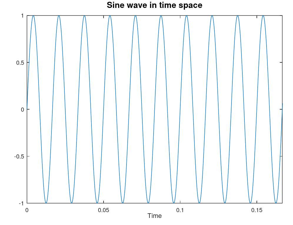	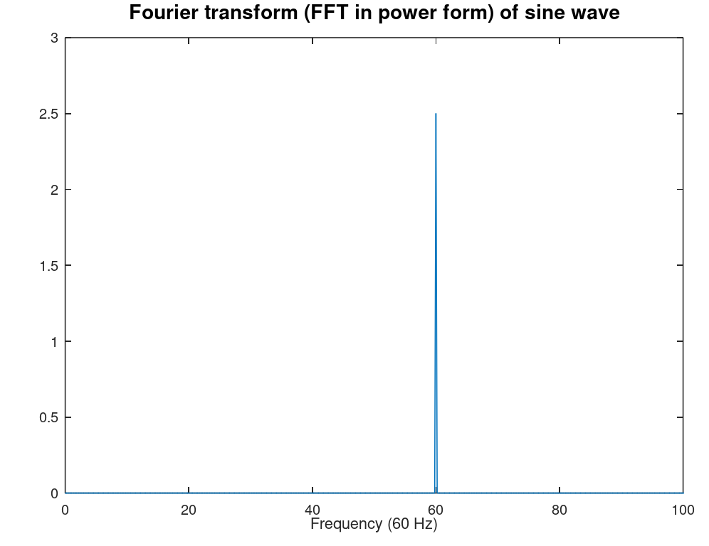A graph is not very meaningful here
Digital Form	Vector array	Fast Fourier Transform (FFT)	Z-transform

Contributors and Attributions

• Franz S. Hover & Michael S. Triantafyllou
• Some modification of this section, particularly the last two tables, were done by Scott D. Johnson, Joshua Halpern, and Scott Sinex. The majority of the work is however Hover's and Triantafyllou's

---

¹Causal systems only depend on present and past. Non-causal systems have a future component which would not be found in the real world, but in data processing we might be able to use future values to process present values (post-processing).