
14.9: Statistics and Probability
- Page ID
- 45263
Statistics is the collecting and analyzing of numerical data for the purpose of inferring results from representative samples sometimes referred to as statistical analysis. Probability quantifies how likely an event is to occur given certain conditions. Given a random variable R we can define some basic principals of probability. P(R) will represent the probability of a random event R will occur.
- \(P(R) \geq 0\)
- \(\sum_i P(R_i) = 1.0\)
- For random variables Q and R: \(P(Q \cup R) = P(Q) + P(R) - P(Q \cap R)\)
- For random variables Q and R: If the events do not take place in at once then \(P(Q \cap R) = 0\)
- For random variables Q and R: Bayes Theorem: \(P(Q | R) = \frac{P(R | Q) P(Q)}{P(R)}\) where \((Q | R)\) means Q given R
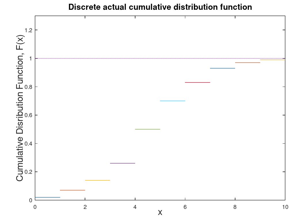
Here let us assume there is a random variable R which is associated with a number or a range of numbers within a given probability distribution. Lets assume we have we have \(x_i\) numbers (let say the score for a quiz that is worth 10 points). Let us define a function F(x) which will be our cumulative distribution function (CDF). The CDF will by the probability that a random variable is less than a specific value of x (in this case 10). The range of F(x) is from 0 to 1 (which is a bit obvious, eh?). Theoretically \(F(-\infty)\) = 0 and increases with each larger value of x.
| Discrete | Continuous |
|---|---|
 |
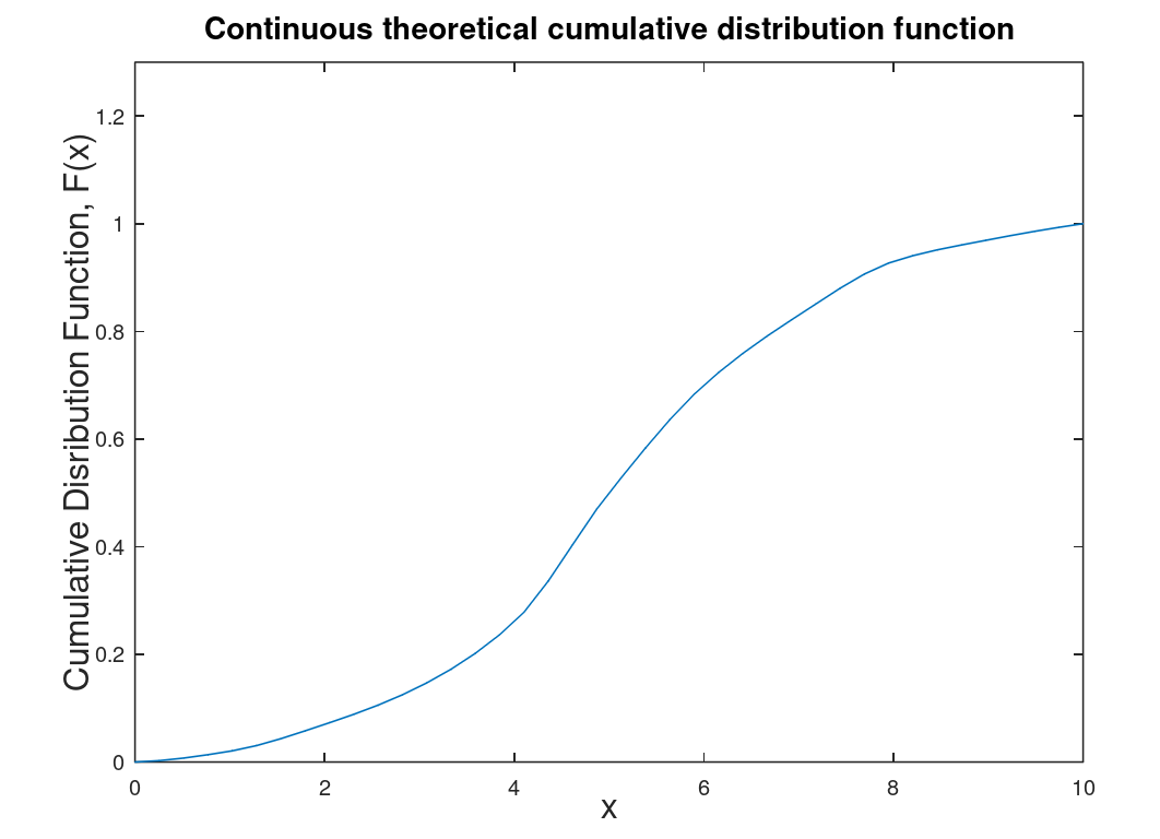 |
| Discrete cumulative distribution function (CDF) which is determined through data either collected or experimental. | Continuous CDF which is theoretical and derived from the discrete CDF. To determine the probability that R lies between \(x_1\) and \(x_2\) use the following formula: \(P(x_1 \leq R < x_2) = F(x_2)-F(x_1)\) |
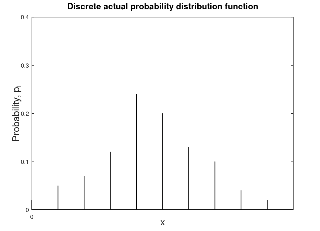
Of more use is the probability distribution function (PDF) which is the particular probability of the random variable R at \(x_i\).
| Discrete | Continuous |
|---|---|
 |
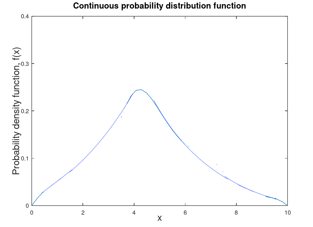 |
| Discrete probability distribution function (PDF) which is based of collected or experimental data as is the discrete CDF. This is referred to as the probability mass function (PMF). | Continuous PDF which is theoretical and derived from the discrete PDF. To determine the probability that R lies between \(x_1\) and \(x_2\) is the area under the curve between those values or \(P(x_1 \leq R < x_2) = \int_{x_1}^{x_2} f(x) dx\). This is technically referred to as the probability density function (PDF) though it is also referred to as the probability distribution function (which is actually more general and includes CDF and PMF). |
With the PDF we can define quantities like mean and variance.
| Discrete (mean and variance) | Continuous (expected mean and variance) |
|---|---|
| \(\overline{x} = \sum_{i=1}^n x_i p_i\) | \(\mu = \int_{-\infty}^{\infty} x \cdot f(x) dx\) |
| \(\sigma^2 = \sum_{i=1}^n (x_i - \overline{x})^2 \cdot p_i\) | \(\sigma^2 = \int_{-\infty}^{\infty} (x - \mu)^2 \cdot f(x) dx\) |
Here you can view \(p_i\) as a kind of weight. When you take an average you are taking a mean with a weight of \(\frac{1}{n}\) where n is the number of data points. f(x) can be viewed as kind of a continuous weight. But what weight to use? That is the "science" to this as there are many statistical distributions that could be used which depends on the system (or experiment).
Here we present a table of statistical distributions, statistical coefficients, and statistical models that are used in science and engineering.
| Distribution | Uses | Graph of PDF or a comment | Comparison graph to Gaussian or Poisson PDF or a comment |
|---|---|---|---|
| Gaussian distribution (or error distribution or normal distribution) | Random error. All distributions as n goes to infinity are Gaussian | 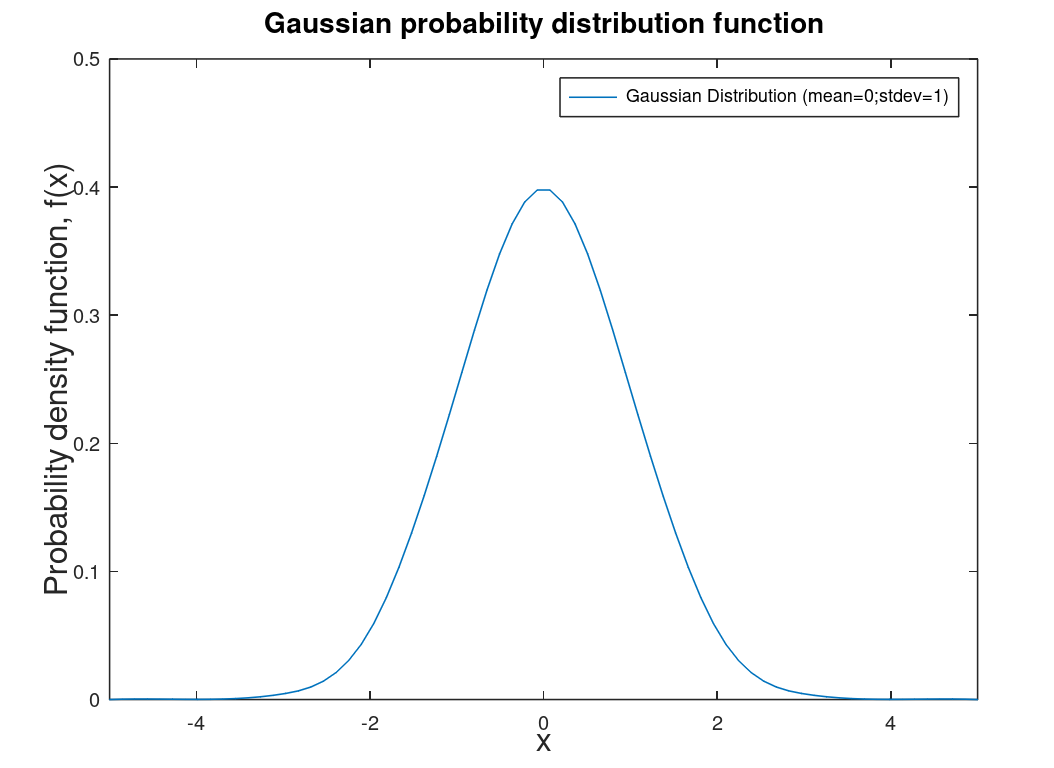 |
This is the distribution that all other distributions tend towards |
| Bimodal distribution | Usually two normal distribution side-by-side, typical of student test grades and heights of humans. (could have more then two distribution then that would be multimodal distribution). | 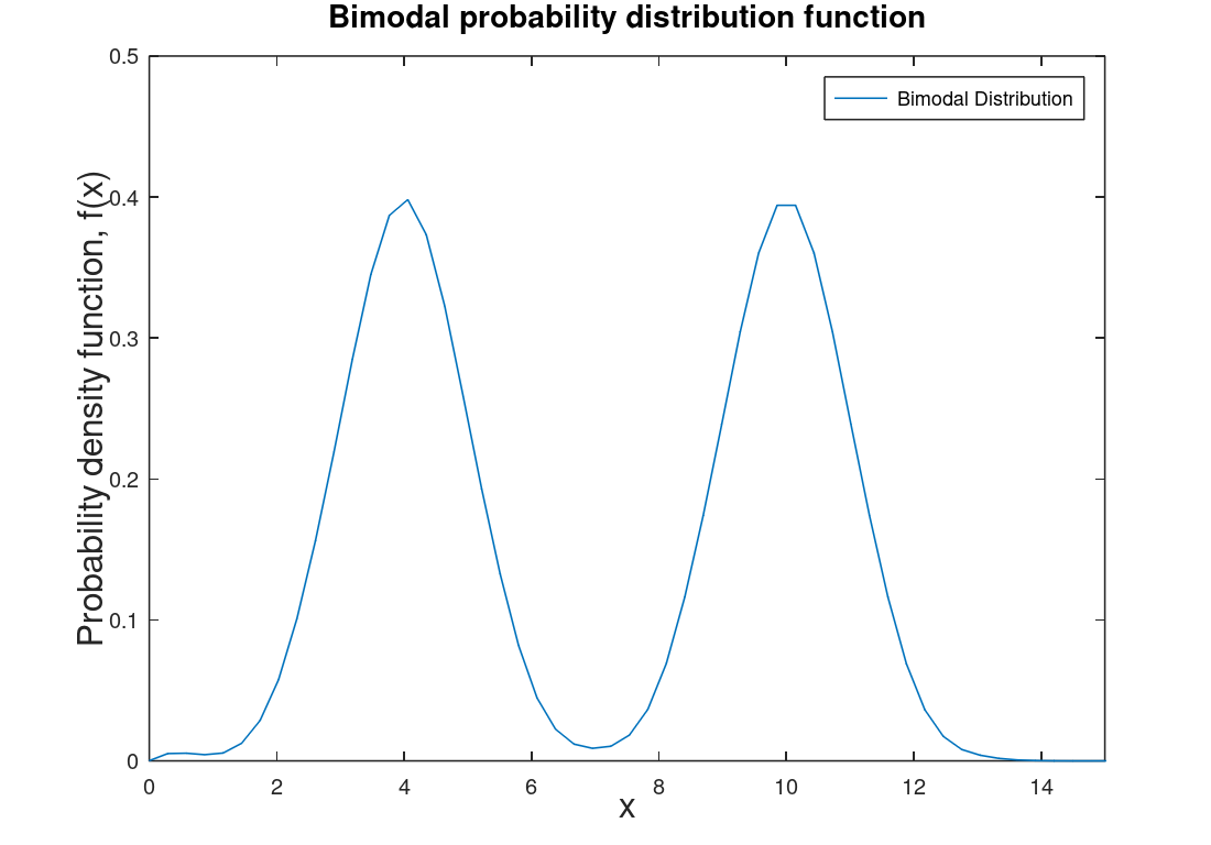 |
Gaussian distributions when more than one distinct group is involved (male human heights and femal human heights when done together). |
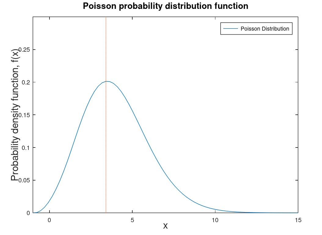
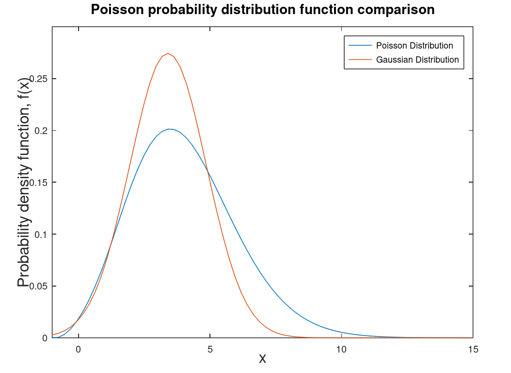
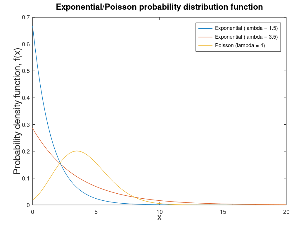
| Poisson distribution |
Counting distribution. Photons on a CCD are described by a Poisson distribution. The graphs at left are the Poisson PDF and a comparison of the Poisson PDF to the Gaussian PDF. Note: counting distributions are integer-based (discrete) so the graph on the right is smoothed for comparison purposes and integration purposes. Discrete distributions are technically PMF (probability mass functions) which are the discrete versions of PDFs. |
 |
 |
| Exponential distribution | Related to the Poisson distribution1 and special case of the Gamma distribution. Used in reliability calculations in engineering. Helps determine the probability of an event's occurrence. Note: Lambda is the rate of events in a particular interval. | 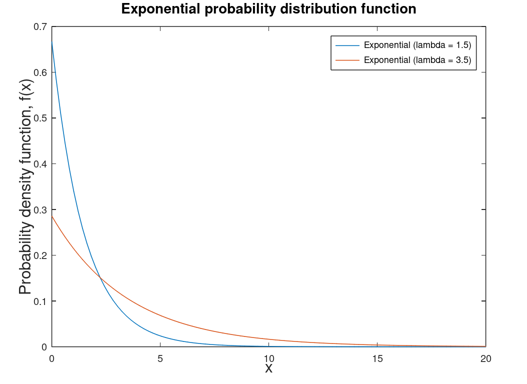 |
 |
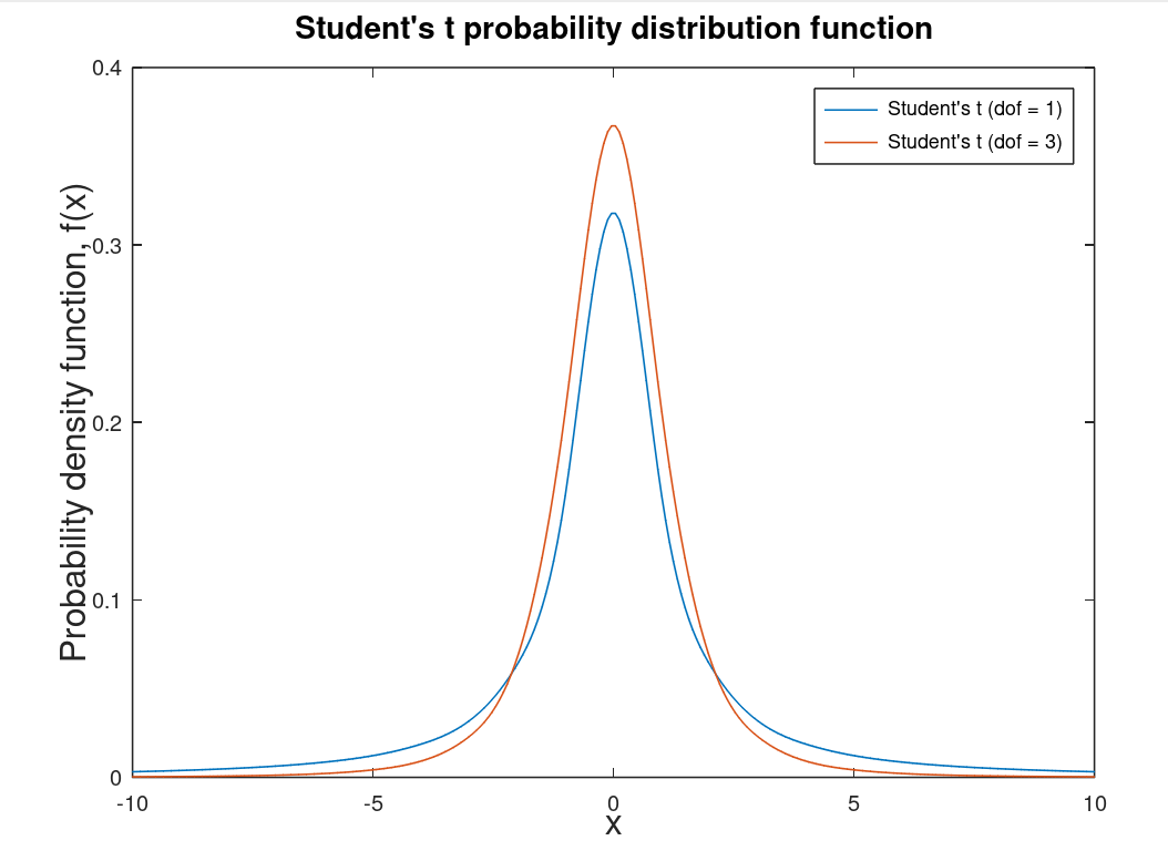
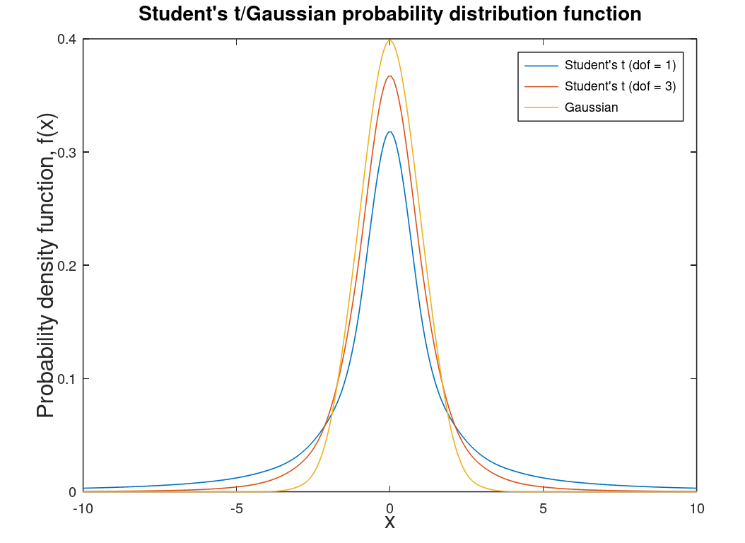
| Student's t-distribution |
A distribution for small statistics2 and unknown standard deviation. Degrees of freedom (dof) are the number of observations minus one. As the degrees of freedom approaches infinity this distribution becomes the Gaussian distribution (as do all distributions). This distribution is associated with the T-Test. |
 |
 |
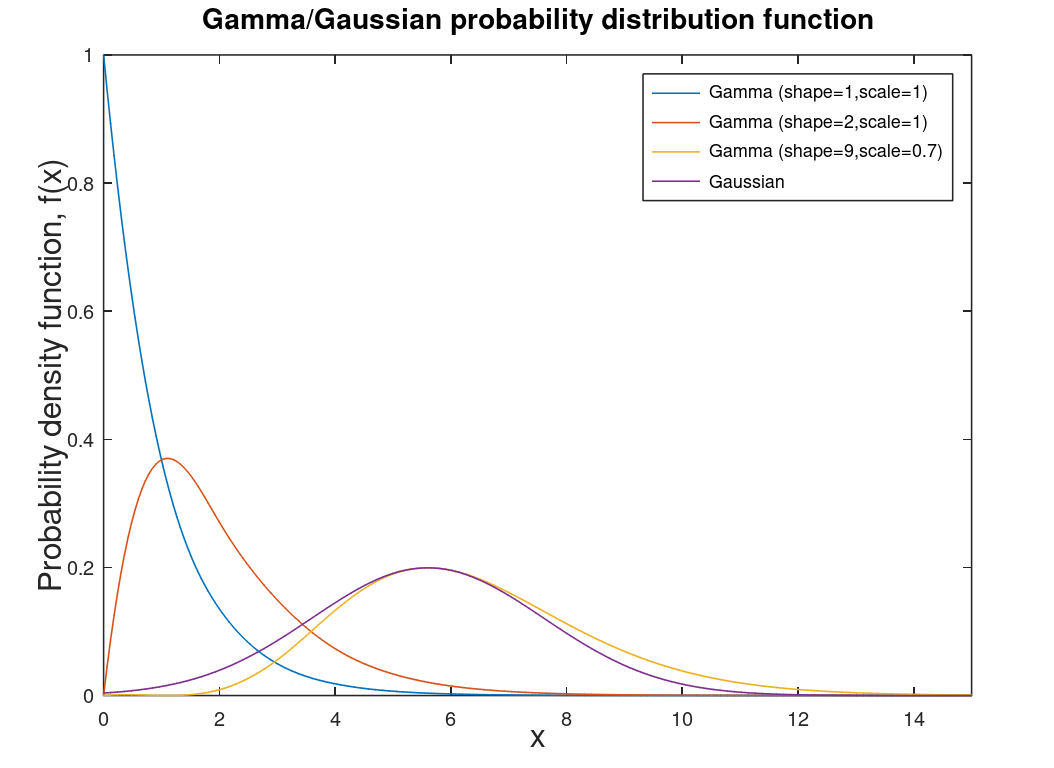
| Gamma distribution | Distribution for modeling errors in different distributions. This distribution is a two parameter distribution that is more a mathematical construct of many other distributions, like chi-square distribution. | 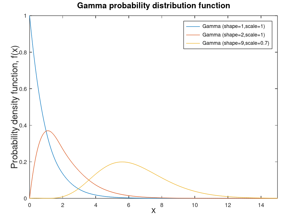 |
 |
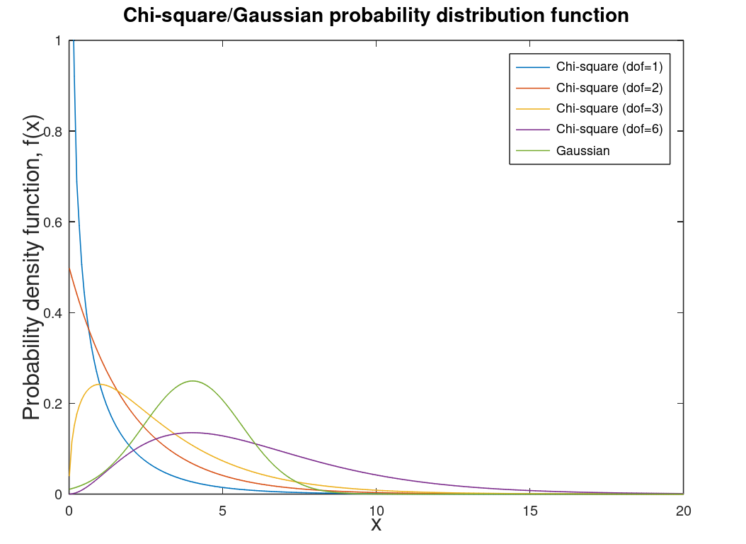
| Chi-square distribution | Special case of gamma distribution. Used for confidence intervals and hypothesis testing (inferential statistics). One of the most used distributions in science, economics, and engineering. | 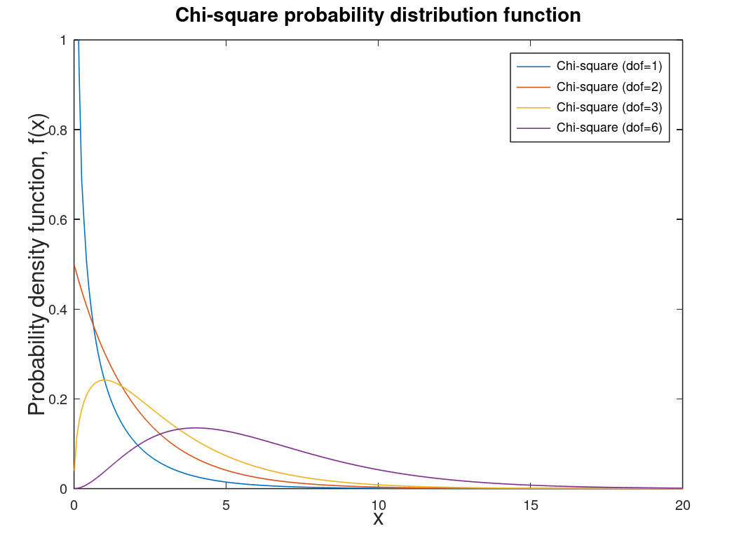 |
 |
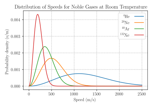
| Maxwellian distribution | Distribution used for velocity distribution in a kinetic gas in physics. |
Maxwellian-Boltzmann Distribution3 |
This is a chi distribution |
| Kappa distribution | A replacement for Maxwellian distribution in certain conditions (non-equilibrium; nonextensive). Useful in statistical mechanics. Maxwellian distribution is special case of the Kappa distribution. | Commonly used for space plasma because space plasma is not in thermal equilibrium. Also used in economics and personal finance. | View this as a deformation of the Maxwellian distribution (of course if the deformation is zero it is the Maxwellian distribution) |
| Cohen's Kappa coefficient | Used to assess the agreement of two raters or to assess classification models. Useful in citizen science like eBird or Zooniverse. | Not a distribution. | Not a distribution. |
| ANOVA | Analysis of variance |
ANOVA4 is a set of models that model the random aspects of a system from its systematic aspects. (One-way ANOVA) Similar tests are the T-Test or Kruskal–Wallis test (which is a modified ANOVA test). Other tests, tests variances instead of means like the F-Test. |
Not a distribution but a model. The test is basically a test of the means of two systems (experiments) using in-group and between group sum of squares (variance without a weight). Null hypothesis means no difference between two systems (experiments). Alternative hypothesis means there is a difference between the two systems (experiments). |
| Factorial ANOVA | N-factor or N-way ANOVA (one of the most common examples is a two-way ANOVA). | More then one independent variable ANOVA. Two-way would be two independent variables, three-way would be three independent variable, etc. | ANOVA is used to test if independent groups have significant differences. \(N\) or more independent groups defined by \(N-1\) independent variables. |
| F distribution | Distribution associated with analysis of variance (ANOVA) and F-Test. This distribution can be described as skewed5. | 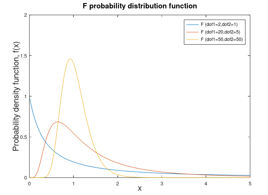 |
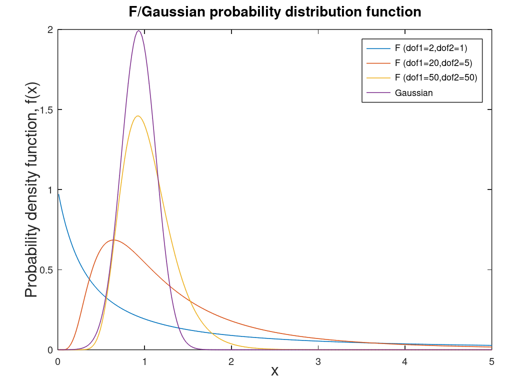 |
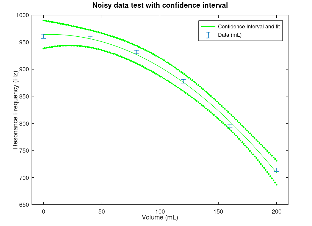
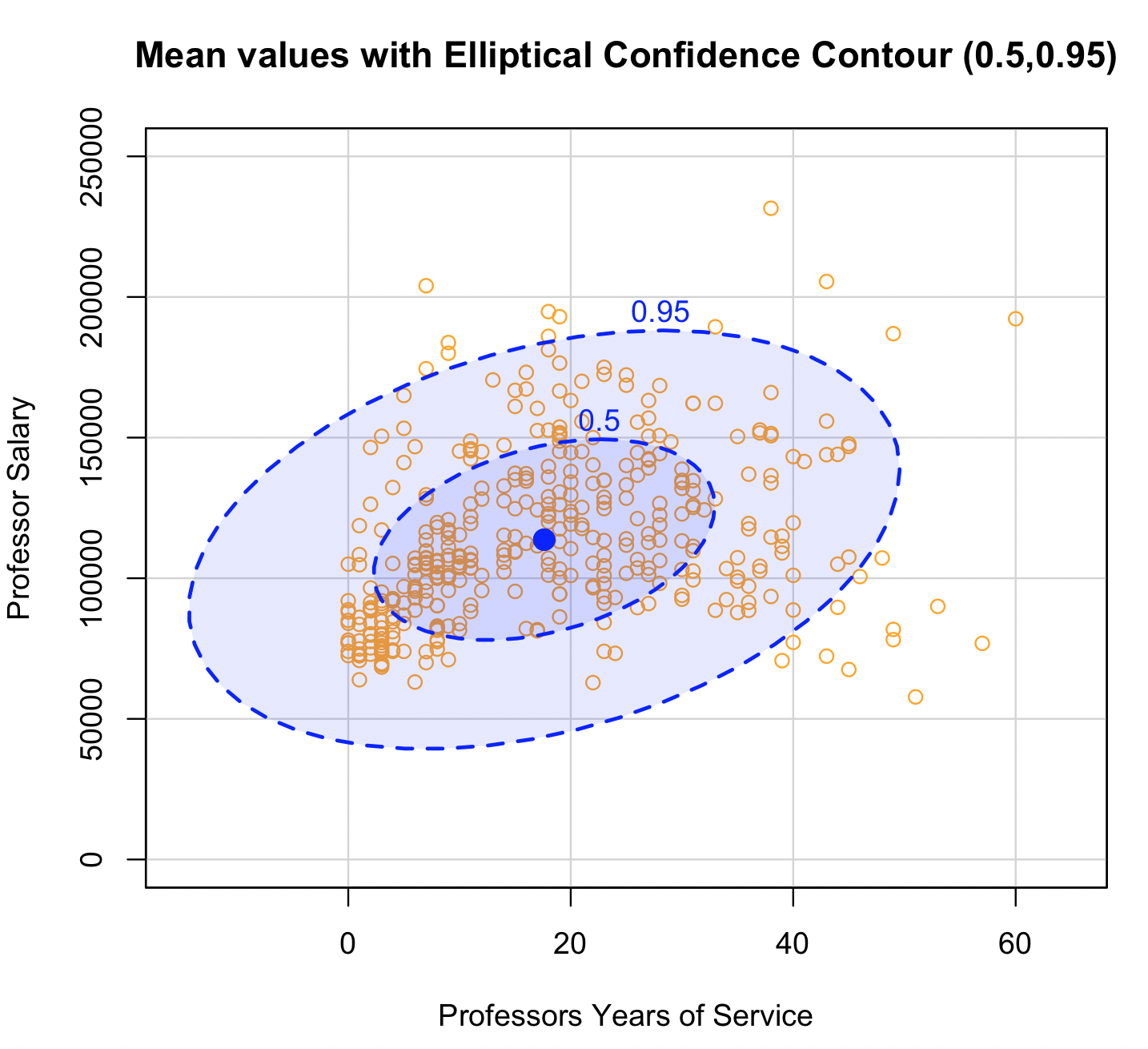
| Confidence interval or confidence contour |
Given that a data's probability distribution is known or can be approximated, the confidence interval or contour line (2D) represents the probability of the data being inside the interval or contour line. The confidence level is specified by the analyst (95% is a typical value). This is not a distribution. |
 |
Confidence Contour using the R programming language6
|
This concludes the brief introduction to statistics and probability. It is highly encouraged for you to take a calculus-based probability course in you junior or senior year of university. Many details left out of this brief introduction will be filled in. The next discussion will be about the all important subject of differential equations in brief.
1Technically the Poisson point process which is a mathematical structure of random variables. It looks remarkable like queueing theory for arrival times, etc. From an engineering point of view it is mostly important for reliability.
2It is important to understand that small statistics can be biased, in particular standard deviations (and hence or "normal" error) can be smaller with a small sample compared to a larger sample. Student t would work to resolve that bias by weighing the points differently.
3Public domain image of speeds of noble gases at room temperature from Wikipedia.
4Using ANOVA with the R programming language (S programming language made new "again." This language was influenced by the one of the most unusual languages - APL) is described in the Libretexts' course: Learning Statistics with R - A tutorial for Psychology Students and other Beginners by Navarro.
5Skewness is a statistical measurement like mean that describes how your data or PDF is skewed in relationship to a normal (Gaussian) curve. This is different from Kurtosis which describes the strength of your tail in your data or PDF compared to a normal (Gaussian) curve.
6This is a confidence contour using the R programming language (S programming language made new again) and the car package with the carData package that contains data (which we used here) that are licenses under GNU General Public License v2.0. R is a language that centers around statistical analysis, so it is worth taken a look at...it's free so go for it.