14.14: Signals and Systems (Control systems)

Signals and Systems

"Signals and systems" is the study of processes with signal input(s) and signal output(s). The methods of this is applicable to all engineering disciplines. Therefore all engineers should take a course in signals and systems. So what is a signal? and what is a system?

A signal is the representation of a physical "wave" expressed as a variable in time-space (example: x(t)). Signals may be voltage or current of a circuit, the force in a mechanical circuit, heat flow in a thermal circuit, or hydraulic flow in a fluid circuit. It is likely this is familiar to the student already so as a challenge to the student: find ten more examples of signals in engineering or science.

A system is a process that has an input a signal or signals and outputs a different signal or signals (usually). A system is generally expressed as a transfer function or an operator. An example of this would be an integrator that integrates the input signal over time as its output. Another more simple example might be an operator that just multiplies the signal by a constant and outputs that new signal.

The methods that are used for the systems are in general the same methods generally learned in linear algebra. The methods used to model the physical aspects of the "signals" are the same methods generally learned in numerical methods.

A system can be expressed mathematically as a transfer function or an operator. A simple example of an operator could be an integrator that takes a signal and integrates it over time or it could be as simple as adding a constant to a signal. Transfer functions are specific to engineering and have the notation of a Laplace transform, where as operators are more specific to physics (and other sciences) and have the notation of mathematics. In the following figure are some examples of how engineers express this symbolically.

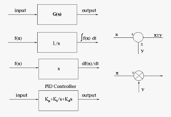In this figure are examples of blocks that represent transfer functions. The signal is the input and the output and inside the block is the transfer function, represented by G(s) in the first example. The s-space notation is consistent with Laplace transformations. The blocks other than the first general block shows examples of how the blocks might be used in a diagram.

Simple Example: Signals and Systems

Let us imagine we are standing in a heavy wind and we are almost blown over. In this instance our brain, through our skin sensors and our muscles, detect that the wind is putting us in a metastable state that could lead to us falling over. So the brain (our controller) sends a message to the muscles and tells them to adjust our position to lean into the wind saving us from falling. So let us look at this from the point of view of signals and systems. The wind is a signal as well as our skin sensor and our muscles communication to the brain; our systems are our body, our controller (brain), and our muscles (a muscle acts as a senor and actuator).

In the following table we look at a conceptual block diagram of the system described above and then look at the conversion of that to a transfer function block diagram that is consistent with control system concepts that engineers generally use.

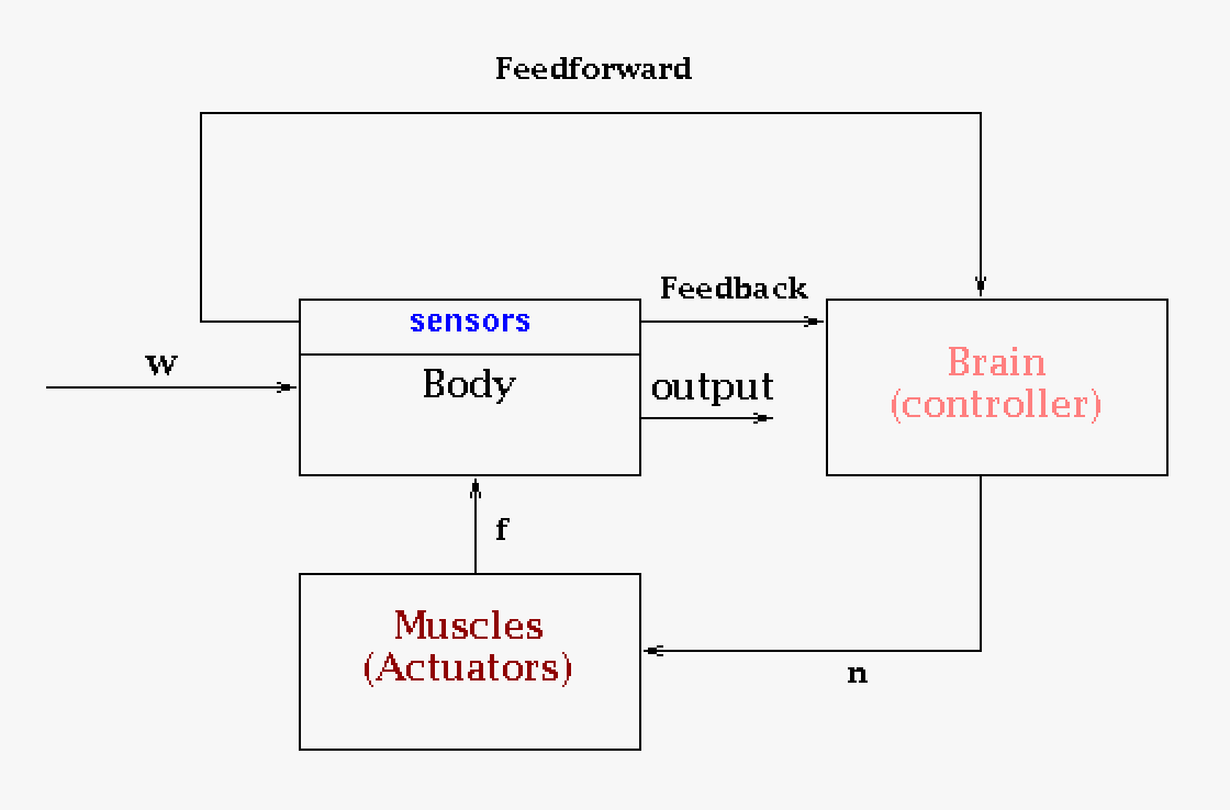
In this conceptual block diagram the body is a system of muscles and skeleton that represent our structure (this could equally well be a building), the control system that takes feedback from sensors is the brain and the brain through a neural network instructs the muscles (actuators) what to do. The main input is the wind, w, but within the block diagram there are also inputs of force, f, and neural net input, n. The sensors for the eyes, muscles, ears, and skin. The eyes can predict wind coming our way and correct our body (by maybe leaning it into the wind) as a preparation. The eyes give us feedforward information which for the transfer function block diagram we will ignore (feedforward is complicated is generally avoided the same reason as extrapolation is avoided in science). For our feedback system we have the skin as a pressure sensor, the ears as a balance sensor, and the muscles are strain sensors. Feedback is crucial in designing a control system.

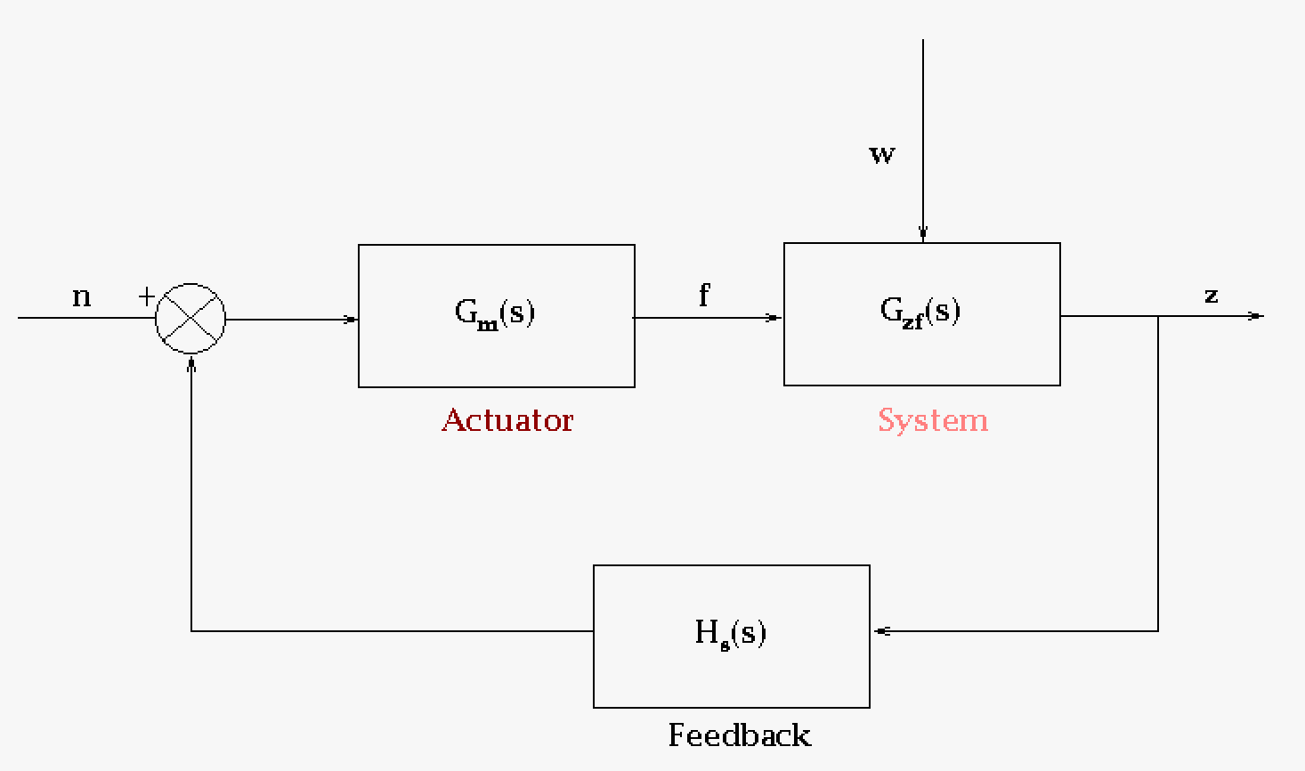
This is a transfer function block diagram that gives the engineers a design to work with. Transfer functions are operators and describe exactly how an input will be transferred into an output. The transfer function is usually a vector or matrix structure that usually have differential equation that act as operators. For a structure the basis of the differential equation will be a force equation \(\mathbf{M_s} \mathbf{\ddot{x}} + \mathbf{C_s} \mathbf{\dot{x}} + \mathbf{K_s} \mathbf{x} = \boldsymbol{\beta_s} f + ...\). The variables are bold here because they are matrices. And yes, this is a matrix of differential equations. A structure is complex and would require a number of differential equations which would need to be solved with matrix mathematics (possibly sparse). Laplace formalism would convert the differential formalism into an algebraic form which would allow for easier calculations, possibility. Note that the force equation could be an equation in another discipline just as well due the idea of dynamic analogies. See next section.

This is just a brief look at control systems and the use of transfer functions. More formal descriptions would happen in your Signals and Systems course (which hopefully would have some Numerical Methods discussion).

Bode Plots (Nyquist plots and Nichols plots)

Bode plots are frequency response plots of a system described by the transfer function. Bode plots consist of both a magnitude plot and a phase plot help to characterize the stability of the system through gain, gain margin, and phase margin. The are very important in system analysis.

Nyquist plots are similar to the Bode plots but in a different coordinate systems ("polar"). Nichols plot is a different form of a Bode plot. For a simple transfer function we will look at a mass, damper, and spring system: \(G(s) = \frac{1}{ms^2+cs+k}\)

pkg load control
T = tf([1],[5 4 3])
bode(T)
figure(2)
nyquist(T)

The output of this simple systems shows an stable oscillatory system. Nothing very noteworthy, but for more complicated systems this can be very helpful. Again if you want more detail check out your Signals and Systems course.

Dynamic Analogies Discussion

We use generic transfer function descriptions when modeling systems rather than discipline specific symbols because of the idea of dynamic analogies. The idea is that the systems of one discipline can be used in other disciplines. Below we give a simple example of this idea and then a incomplete table of analogies (enough to give an idea which should be pursued more fully in later classes).

This model is based off the comparison that \(F=\frac{dp}{dt}=m\frac{dv}{dt}\) and \(I=C\frac{dV}{dt}\) where force¹ is to be associated with current and velocity with voltage. That leads to the idea that mass is associated with capacitance. Similarly with the equation \(I=\frac{1}{L}\int{V dt}\) the spring constant, K, is to be associated with 1/L and with the equation \(I = \frac{1}{R} V\) the damping coefficient, B, is associated with 1/R.

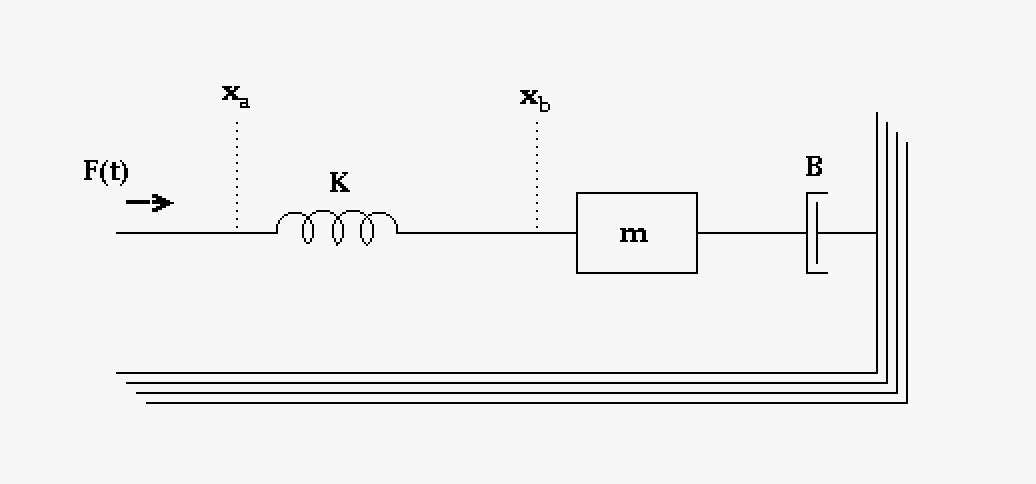	This is a system that includes a spring, a mass, and a damper. K is the spring constant, m is the mass, and B is the damping coefficient. A force is being applied on this system F(t). This is the system we wish to use as a system model. Many mechanical process can be described by these three elements.
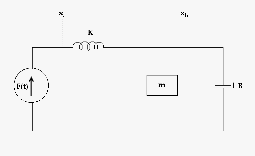	This takes the above system and converts it to a mechanical circuit which is a convenience that will help us going to the next step.
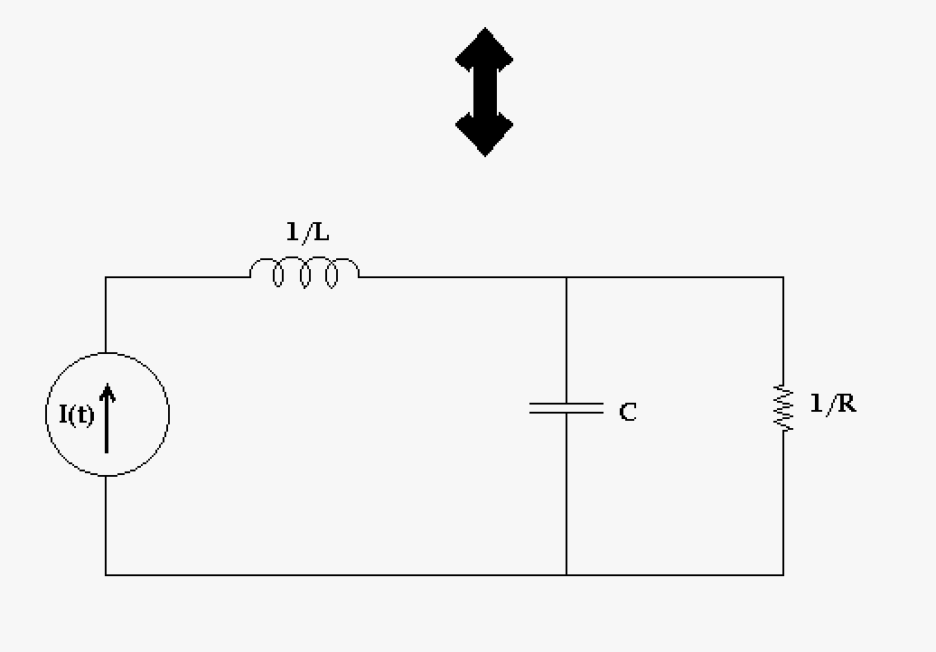	This is the equivalent electrical circuit that would emulate the above mechanical circuit. Mechanical circuits might describe systems that are very large, however converting them into an electric circuit would make a physical simulation easier. Alternatively this could be run in a Spice, which would then make the electronic simulator into an mechanical simulator.

The following table gives a list of some equivalencies to different physical system. Traditionally these are call dynamical analogies. Different ways to create models will change this list so this is not an all encompassing list. There are many missing analogies here as, again, this is not meant to be complete.

Mechanical	Electrical	Thermal	Hydraulic	Mechanical - rotational
Force, F	Current, I	Rate of heat flow, q	Volumetric flow rate, Q	Torque, \(\tau\)
Velocity, v	Voltage, V	Temperature (\(\theta\))	Pressure, P	Angular velocity, \(\omega\)
Mass, m	Capacitance, C	Thermal capacitance (C = mc)	Tank area, AT	Moment of inertia, I
Spring constant^2, K	1/L	-	-	Torsion spring constant^2, \(\kappa\)
Damping coefficient, B	1/R	-	Flow conductivity, K	Rotational damping coefficient, D
-	Capacitor voltage, Vc	-	Liquid height, h	-
-	Resistance, R	Thermal resistance, R	Flow resistance, R	-
Momentum, p	-	heat	-	Angular momentum, L
-	-	Specific heat, c	-	-

From an energy perspective these analogies are more obvious and it is one reason you will find Lagrangian and Hamiltonian methods used in physics.

Signals and Systems Concluded

Signals and systems really describe a large number of engineering and science process. The brief discussion here is to show you what this is all about, but is definitely not complete. For an introduction in engineering class this is more then enough so we will move on to the next topic.

---

¹Alternatively we could look at force as associated with voltage which would change the electrical analogs correspondingly. We believe that force and current are are better analogies then force and voltage. Voltage is a difference which is more like how velocity is defined with dx.

²From a dynamical analogy point of view whether this is a spring coefficient or stiffness coefficient is not material as it still would be represented by a spring. This is similar for the torsion spring coefficient or rotational stiffness coefficient.