1.8: Deeper Questions

1. A specimen of sheet steel is tested in unequal biaxial tension, and Lüders bands form at 60° to one of the tensile axes. Show that the ratio between the two principal stresses in the plane of the sheet is 1:5.

If the greater of these two principal stresses is 500 MPa and the steel obeys von Mises' yield criterion, show that the yield stress in uniaxial tension is 458 MPa.

Answer

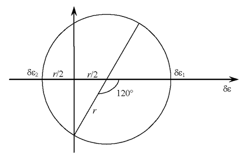
If the specimen is tested in unequal biaxial tension, we have stresses and which give rise to strain increments \(\delta \varepsilon_{1}\) and \(\delta \varepsilon_{2}\). As before the longitudinal plastic strain along the Lüders band has to be zero. We first use Mohr’s circle to calculate the ratio of \(\delta \varepsilon_{1}\) to \(\delta \varepsilon_{2}\):

Now, cos 120° = – \(\frac{1}{2}\), and so the centre of the Mohr’s circle must be \(\frac{r}{2}\) to the right of zero. Therefore, \(\delta \varepsilon_{2}\) must be \(\frac{r}{2}\) to the left of zero and \(\delta \varepsilon_{1}\) must be \(\frac{3r}{2}\) to the right of zero.

Hence, \(\delta \varepsilon_{1}=-3 \delta \varepsilon_{2}\).

Using the Lévy-Mises equations, we have:

\[\frac{\delta \varepsilon_{1}}{\sigma_{1}-\frac{1}{2} \sigma_{2}}=\frac{\delta \varepsilon_{2}}{\sigma_{2}-\frac{1}{2} \sigma_{1}}\]

and so if \(\delta \varepsilon_{1}=-3 \delta \varepsilon_{2}\), we have:

\[-3\left(\sigma_{2}-\frac{1}{2} \sigma_{1}\right)=\left(\sigma_{1}-\frac{1}{2} \sigma_{2}\right)\]

and so \(\sigma_{1}=5 \sigma_{2}\).

If \(\sigma_{1}\) = 500 MPa, it follows that \(\sigma_{2}\) = 100 MPa.

If is the yield stress in uniaxial tension, it follows from the von Mises yield criterion that

\[\left(\sigma_{1}-\sigma_{2}\right)^{2}+\sigma_{2}^{2}+\sigma_{1}^{2}=2 Y^{2}\]

for this situation since If = 0. Hence working in units of \(\sigma_{2}\), we have:

\[16 \sigma_{2}^{2}+\sigma_{2}^{2}+25 \sigma_{2}^{2}=2 Y^{2}\]

and so

\[Y=\sqrt{21} \sigma_{2}=4.58 \sigma_{2}=458 \mathrm{MPa}(3 \mathrm{s.f.})\]

2. Use a work formula approach to estimate the minimum pressure required to extrude aluminium curtain rail of I-section, 12 mm high with 6 mm wide flanges, all 1.6 mm thick, from 25 mm diameter bar stock.

[The mean uniaxial yield stress for aluminium for heavy deformation at room temperature is 150 MPa. The minimum pressure, \(p_{min}\), required is given by the formula

\[p_{\mathrm{min}}=Y \ln \left(\frac{A_{0}}{A_{1}}\right)\]

where \(A_0\) is the original cross-sectional area and \(A_1\) is the cross-sectional area of the extruded I-section].

Answer

From the data given,

\[A_{0}=\pi\left(\frac{25}{2}\right)^{2} \mathrm{mm}^{2}\]

and

\[A_{1}=(2 \times 6 \times 1.6)+((12-2 \times 1.6) \times 1.6) \mathrm{mm}^{2}=33.28 \mathrm{mm}^{2}\]

Hence,

\[R=\frac{A_{0}}{A_{1}}=14.75\]

Therefore,

\[p_{\mathrm{min}}=150 \ln (14.75)=404 \mathrm{MPa}\]

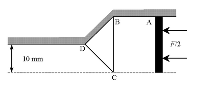
3. The diagram below shows a possible deformation pattern for the direct plane-strain extrusion of a metal slab, initially 40 mm thick, through a symmetrical 45° tapering die, with an extrusion ratio of 2.The diagram shows half the deformation pattern and the angles BCD and CBD are both 45°. The distance AB is 15 mm. The width of the slab is 100 mm and its yield stress in pure shear is 150 MPa.

Calculate an upper bound to the extrusion force F acting on the slab if the extrusion process is frictionless.

Hint:

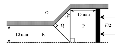
Begin by labelling the various regions of the diagram showing direct extrusion:

O is a stationary component of the system. The hodograph is straightforward for this special geometry:

Answer

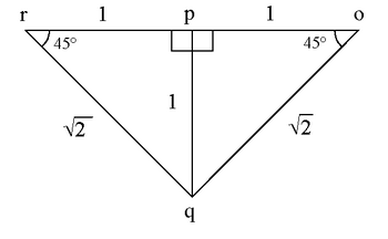
If the extrusion process is frictionless, energy is only dissipated on PQ and QR, so applying the usual work formula, we have, per unit depth into the plane of the paper,

\[\frac{F}{2} \cdot \mathrm{op}=k(\mathrm{PQ} \cdot \mathrm{pq}+\mathrm{QR} \cdot \mathrm{qr})\]

Now op = pq = 1 and qr = \(\sqrt{2}\), PQ = 20 mm and QR = \(10\sqrt{2}\) mm, so

\[\frac{F}{2}=k(20.1+10 \sqrt{2} . \sqrt{2}) \times 10^{-3}=40 \times 10^{-3} k\]

per unit depth, with lengths in metres.

Hence, for a 100 mm wide slab whose yield stress, \(k\), in pure shear is 150 MPa,

\[F=\left(80 \times 10^{-3}\right) \times\left(150 \times 10^{6}\right) \times\left(100 \times 10^{-3}\right) \mathrm{N}=1.2 \mathrm{ MN}\]