30.4: Enforcing Boundary Conditions

Last updated
Save as PDF

Page ID: 32863

\( \newcommand{\vecs}[1]{\overset { \scriptstyle \rightharpoonup} {\mathbf{#1}} } \) \( \newcommand{\vecd}[1]{\overset{-\!-\!\rightharpoonup}{\vphantom{a}\smash {#1}}} \)\(\newcommand{\id}{\mathrm{id}}\) \( \newcommand{\Span}{\mathrm{span}}\) \( \newcommand{\kernel}{\mathrm{null}\,}\) \( \newcommand{\range}{\mathrm{range}\,}\) \( \newcommand{\RealPart}{\mathrm{Re}}\) \( \newcommand{\ImaginaryPart}{\mathrm{Im}}\) \( \newcommand{\Argument}{\mathrm{Arg}}\) \( \newcommand{\norm}[1]{\| #1 \|}\) \( \newcommand{\inner}[2]{\langle #1, #2 \rangle}\) \( \newcommand{\Span}{\mathrm{span}}\) \(\newcommand{\id}{\mathrm{id}}\) \( \newcommand{\Span}{\mathrm{span}}\) \( \newcommand{\kernel}{\mathrm{null}\,}\) \( \newcommand{\range}{\mathrm{range}\,}\) \( \newcommand{\RealPart}{\mathrm{Re}}\) \( \newcommand{\ImaginaryPart}{\mathrm{Im}}\) \( \newcommand{\Argument}{\mathrm{Arg}}\) \( \newcommand{\norm}[1]{\| #1 \|}\) \( \newcommand{\inner}[2]{\langle #1, #2 \rangle}\) \( \newcommand{\Span}{\mathrm{span}}\)\(\newcommand{\AA}{\unicode[.8,0]{x212B}}\)

By enforcing boundary conditions, such as those depicted in the system below, [K] becomes invertible (non-singular) and we can solve for the reaction force F₁ and the unknown displacements u₂ and u₃, for known (applied) F₂ and F₃.

alt

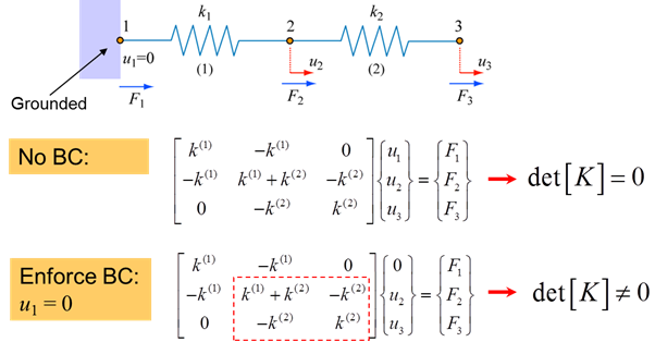
\[ [K] =
\begin{bmatrix}
k^1 + k^2 & -k^2\\
-k^2 & k^2
\end{bmatrix}
=
\begin{bmatrix}
a & b\\
c & d
\end{bmatrix} \]

\[ det[K] = ad - cb \]

\[ det[K] = (k^1 + k^2)k^2 - {k^2}^2 = k^1k^2 \neq 0 \]

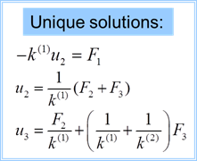
Unique solutions for \(F_1\), \(\begin{Bmatrix}u_2\end{Bmatrix}\) and \(\begin{Bmatrix}u_3\end{Bmatrix}\) can now be found

\[ k^1u_2 = F_1\]

\[ (k^1+k^2)u_2 - k^2u_3 = F_2 = k^1u_2 + k^2u_2 - k^2u_3 \]

\[ -k^2u_2 + k^2u_3 = F_3 \]

Unique solutions

In this instance we solved three equations for three unknowns. In problems of practical interest the order of \([K]\) is often very large and we can have thousands of unknowns. It then becomes impractical to solve for \(\begin{Bmatrix}u\end{Bmatrix}\) by direct inversion of the global stiffness matrix. We can instead use Gauss elimination which is much more suitable for solving systems of linear equations with thousands of unknowns.

Gauss Elimination

We have a system of equations

\[x - 3y + z = 4\]

\[2x - 8y + 8z = -2\]

\[-6x + 3y -15z = 9\]

We wish to create a matrix of the following form

\[\begin{bmatrix}1 & -3 & 1 & 4 \\ 2 & -8 & 8 & -2 \\ -6 & 3 & -15 & 9 \end{bmatrix}\]

\[\begin{bmatrix}11 & 12 & 13 & 1 \\ 0 & 22 & 23 & 2 \\ 0 & 0 & 33 & 3 \end{bmatrix}\]

Where the terms below the direct terms are zero. We need to eliminate some of the unknowns by solving the system of simultaneous equations. To eliminate x from row 2 (where R denotes the row)

-2(R1) + R2

\[ -2(x -3y +z) + (2x - 8y + 8z) = -10 \]

\[ -2y + 6z = -10 \]

so that

\[\begin{bmatrix}1 & -3 & 1 & 4 \\ 0 & -2 & 6 & -10 \\ -6 & 3 & -15 & 9 \end{bmatrix}\]

To eliminate x from row 3

6(R1) + R3

\[ 6(x -3y +z) + (-6x - 3y - 15z) = 33 \]

\[ -15y - 9z = 33\]

\[\begin{bmatrix}1 & -3 & 1 & 4 \\ 0 & -2 & 6 & -10 \\ 0 & -15 & -9 & 33 \end{bmatrix}\]

To eliminate y from row 2

R2/2

\[ -y + 3z = -5\]

\[\begin{bmatrix}1 & -3 & 1 & 4 \\ 0 & -1 & 3 & -5 \\ 0 & -15 & -9 & 33 \end{bmatrix}\]

To eliminate y from row 3

R3/3

\[-5y - 3z = -11\]

\[\begin{bmatrix}1 & -3 & 1 & 4 \\ 0 & -1 & 3 & -5 \\ 0 & -5 & -3 & 11 \end{bmatrix}\]

And then

-5(R2) + R3

\[ -5(-y +3z) + (-5y - 3z) = 36 \]

\[-18z = 36\]

\[\begin{bmatrix}1 & -3 & 1 & 4 \\ 0 & -1 & 3 & -5 \\ 0 & 0 & -18 & 36 \end{bmatrix}\]

\[-2 = z\]

Substituting z = -2 back in to R2 gives y = -1

Substituting y = -1 and z = -2 back in to R1 gives x = 3

This process of progressively solving for the unknowns is called back substitution.