2.4: Derivation of the anisotropy ellipsoid

Last updated
Save as PDF

Page ID: 7789

\( \newcommand{\vecs}[1]{\overset { \scriptstyle \rightharpoonup} {\mathbf{#1}} } \) \( \newcommand{\vecd}[1]{\overset{-\!-\!\rightharpoonup}{\vphantom{a}\smash {#1}}} \)\(\newcommand{\id}{\mathrm{id}}\) \( \newcommand{\Span}{\mathrm{span}}\) \( \newcommand{\kernel}{\mathrm{null}\,}\) \( \newcommand{\range}{\mathrm{range}\,}\) \( \newcommand{\RealPart}{\mathrm{Re}}\) \( \newcommand{\ImaginaryPart}{\mathrm{Im}}\) \( \newcommand{\Argument}{\mathrm{Arg}}\) \( \newcommand{\norm}[1]{\| #1 \|}\) \( \newcommand{\inner}[2]{\langle #1, #2 \rangle}\) \( \newcommand{\Span}{\mathrm{span}}\) \(\newcommand{\id}{\mathrm{id}}\) \( \newcommand{\Span}{\mathrm{span}}\) \( \newcommand{\kernel}{\mathrm{null}\,}\) \( \newcommand{\range}{\mathrm{range}\,}\) \( \newcommand{\RealPart}{\mathrm{Re}}\) \( \newcommand{\ImaginaryPart}{\mathrm{Im}}\) \( \newcommand{\Argument}{\mathrm{Arg}}\) \( \newcommand{\norm}[1]{\| #1 \|}\) \( \newcommand{\inner}[2]{\langle #1, #2 \rangle}\) \( \newcommand{\Span}{\mathrm{span}}\)\(\newcommand{\AA}{\unicode[.8,0]{x212B}}\)

The variation of anisotropic properties such as conductivity can conveniently be illustrated by a "representation surface". In many cases this is an ellipsoid.

Suppose a three-dimensional temperature gradient, gradT, lies along a direction specified by direction cosines l, m and n>, where, for example, l is the cosine of the angle between the x-axis and the temperature gradient vector. Then the components of the temperature gradient parallel to the principal axes will be:

\[\operatorname{grad} T_{x}=(\operatorname{grad} T) \operatorname{lgrad} T_{y}=(\operatorname{grad} T) \operatorname{mgrad} T_{z}=(\operatorname{grad} T) n\]

The components of the heat flux are:

\[j_{x}=k_{1}(\operatorname{grad} T) l j_{y}=k_{2}(\operatorname{grad} T) m j_{z}=k_{3}(\operatorname{grad} T) n\]

where k₁, k₂ and k₃ are the values of thermal conductivity along the principal axes, x, y and z, and are called the principal values.

Hence, resolving back along the direction of the temperature gradient, the heat flux is:

\[j_{\|}=j_{x} l+j_{y} m+j_{z} n=\left(k_{1} l^{2}+k_{2} m^{2}+k_{3} n^{2}\right) g r a d T\]

Thus the value of the thermal conductivity, k_lmn, defined by

\[k_{l m n}=\frac{j_{\|}}{g r a d T}\]

is related to the principal values and the directional cosines by:

\[k=k_{1} \cdot l^{2}+k_{2} \cdot m^{2}+k_{3} \cdot n^{2}\]

\[l=x / r \quad m=y / r \quad n=z / r\]

Substituting in our equation for k gives:

\[k=\frac{k_{1} x^{2}}{r^{2}}+\frac{k_{2} y^{2}}{r^{2}}+\frac{k_{3} z^{2}}{r^{2}}=\frac{1}{r^{2}}\left(k_{1} x^{2}+k_{2} y^{2}+k_{3} z^{2}\right)\]

Setting

\[r=1 / \sqrt{k}\]

then

\[k>_{1} x^{2}+k_{2} y^{2}+k_{3} z^{2}=1\]

If all the principal values are positive (as they must be for thermal conductivity), then this equation describes the surface of an ellipsoid. The general equation of an ellipsoid (with semi-axes a,b,c) is:

\[\frac{x^{2}}{a^{2}}+\frac{y^{2}}{b^{2}}+\frac{z^{2}}{c^{2}}=1\]

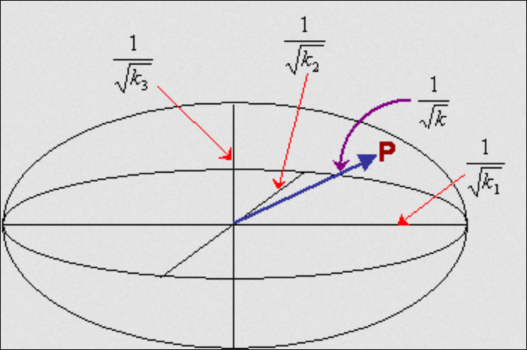
Thus for this representation ellipsoid, the semi-axes are:

\[\frac{1}{\sqrt{k_{1}}}, \frac{1}{\sqrt{k_{2}}}, \frac{1}{\sqrt{k_{3}}}\]

The radius of this ellipsoid in a general direction is equal to the value of \(\frac{1}{\sqrt{k}}\)in that direction. Thus the value of k in a particular direction - the ratio of the component of the heat flow in that direction to the magnitude of the temperature gradient in that direction - can easily be calculated from the radius in that direction.

An equivalent representation surface exists for electrical conductivity, and a similar representation surface exists for refractive index - the optical indicatrix. Both of these are discussed later in this TLP.

Using the representation surface for thermal conductivity

As shown above, the representation surface for thermal conductivity is an ellipsoid with semi-axes \(\frac{1}{\sqrt{k_{1}}}\), \(\frac{1}{\sqrt{k_{2}}}\), and \(\frac{1}{\sqrt{k_{3}}}\). The distance between the centre of the ellipsoid and a point, P, on its surface, is equal to \(\frac{1}{\sqrt{k}}\) at this point.

As well as determing the conductivity, the representation surface can be used to relate the directions of heat flow and the temperature gradient. If the temperature gradient is applied radially from the centre of the ellipsoid, then the direction of resulting heat flow is perpendicular to the tangential plane constructed from the point at which the thermal gradient meets the surface of the ellipsoid.

In an isotropic material, the representation surface will be a sphere, and the heat flow will be in the same direction as the temperature gradient. However, in an anisotropic material, heat flow is no longer necessarily parallel to the temperature gradient.

We will now revisit the anisotropic thermal conductivity of quartz.

Because of the crystal symmetry of quartz, k₁ = k₂ k₃, and so the representation surface for the thermal conductivity of quartz is a uniaxial ellipsoid of revolution. Depending on the relative values of k₁ and k₃, this is a shape either like a rugby ball (k₃ < k₁) or a Smartie (k₃ > k₁).

Consider sections of the ellipsoid:

Since k₁ = k₂, this section is a circle, and the direction of heat flow is parallel to the temperature gradient.
Since k₁ k₃, this section is an ellipse, and the direction of heat flow is no longer parallel to the temperature gradient, except in the directions of the principal axes (which here correspond to the semi-axes of the ellipse).

The direction of the heat flux is always parallel to the normal to the tangential plane drawn at the point at which the direction of the temperature gradient intersects the representation ellipsoid. This is called the radius-normal property.

View proof of the radius-normal property.