
12.3: Constitutive Laws for Creep
- Page ID
- 7859
")
Effects of Microstructure on Creep
As with plastic deformation, creep is a complex process that is strongly affected by the microstructure of the material. (Some of the microstructural effects that influence plasticity are summarised in the TLP on Mechanical Testing.) As with plasticity, however, guidelines can be identified concerning features likely to affect (inhibit) creep, and some of these are similar for the two. For example, a fine array of precipitates, which will inhibit dislocation glide and hence raise the yield stress, is also likely to inhibit (dislocation) creep. However, there are limits to such linkage. For example, precipitates might dissolve at the high temperatures involved in creep. More fundamentally, some features can affect creep and plasticity quite differently. For example, while a fine grain size tends to raise the yield stress, as a result of grain boundaries acting as obstacles to dislocation glide, it can cause accelerated creep in a diffusion-dominated regime, since such boundaries also constitute fast diffusion paths.
Nevertheless, as with plasticity, empirical constitutive laws can be used to model and predict creep behaviour. There is sometimes scope for interpreting the values of parameters in these laws in terms of the dominant mechanisms involved. In particular, if rates of creep are measured over a range of temperature, then it may be possible to evaluate the activation energy, Q (in an Arrhenius expression), which could in turn provide information about the type of diffusional process that is rate-determining. It is also often claimed that the value of a stress exponent, n, obtained via creep rate measurements over a range of applied stress, is indicative of the dominant mechanism, with a low value (~1-2) indicating pure diffusional creep and a higher value (~3-6) suggestive of dislocation creep. The theoretical basis for such conclusions may sometimes be questioned, and in any event these laws must be recognised as essentially empirical, but it is certainly important to be able to characterize the creep response of a material, and to be clear about the regime of temperature and stress for which a particular law is valid.
General (Steady State) Creep Law
The creep strain rate (rate of change of the von Mises plastic strain) in the steady state (Stage II) regime is often written
\[\dot{\varepsilon}=A \sigma^{n} \exp (-Q / R T)\]
where A is a constant, σ is the applied (von Mises - click here for definition) stress, Q is the activation energy and n is the stress exponent. This is a relatively simple equation, but several caveats should be added. The most important of these are apparent in Fig.1 of the Introduction page - ie it relates only to the steady state (secondary) regime. It is sometimes stated that the overall creep life is often dominated by this regime. In practice, this may or may not be true. In particular, it’s worth noting that, not only can the primary regime extend over a significant fraction of the creep lifetime, but also, since the creep rate is often much higher during primary creep, its contribution to the overall creep strain can be substantial, and even dominant. Depending on a number of factors, simply ignoring primary creep may be highly inappropriate.
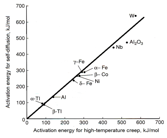
Plot of self-diffusion activation energy vs. high temperature creep activation energy, with a line drawn along which the two are equal. [1]
It may be noted that the activation energy for creep at high temperatures is often found to agree closely with that for bulk diffusion - see, for example, the data in the figure. This is consistent with the concept of N-H creep (diffusion through the lattice) dominating Coble Creep (grain boundary diffusion) at high temperatures.
Laws Capturing both Primary and Secondary Regimes
In view of the potential importance of the primary regime, there is strong interest in using modelling approaches that incorporate it. Several expressions have been proposed for capture of both primary and secondary regimes, and of the transition between them. One that can be taken as representative is the following equation, which is sometimes termed the Miller-Norton law
\[\varepsilon_{\mathrm{cr}}=\frac{C \sigma^{n} t^{m+1}}{m+1} \exp \left(\frac{-Q}{R T}\right)\]
In this expression, C is a constant (units of Pa−n s−(m+1)), t is the time (s), n is the stress exponent and m is a dimensionless constant. The simulation below, in which this equation is plotted, can be used to explore Miller-Norton creep strain plots as the 6 parameters involved are varied.
Simulation showing behaviour predicted by M-N law with constant true stress
A number of features should quickly become apparent, such as the high sensitivity to temperature and that the sensitivity to the applied stress increases as the value of n is raised.
One issue here is whether the applied stress is a nominal or a true value. It certainly should be a true value, as this is implicit in the M-N law. However, it is common during testing to fix the load (often in the form of a dead weight), rather than the true stress. Also, most uniaxial creep tests tend to be carried out in tension. Neglecting any inhomogeneity that might arise, such as a necking effect - which is not common during creep testing - the true stress will rise as straining occurs and the cross-sectional area reduces. Depending on the value of n, this could have the effect of causing the strain rate to rise (whereas it would otherwise be falling and approaching a constant value).
This effect is modeled in the simulation below. The M-N law can be differentiated with respect to time, to give
\[\dot{\varepsilon}_{\mathrm{cr}}=C \sigma^{n} t^{m} \exp \left(\frac{-Q}{R T}\right)\]
Therefore, by stepping in time and repeatedly re-evaluating the true stress, and hence the strain rate, the full creep strain curve can be built up (although it can no longer be expressed as a single analytical equation). In order to implement this, the relationship between true and nominal stresses is needed:
\[\sigma_{T}=\frac{F}{A}=\frac{F L}{A_{0} L_{0}}=\frac{F\left(L_{0}+\varepsilon_{N} L_{0}\right)}{A_{0} L_{0}}=\frac{F}{A_{0}}\left(1+\varepsilon_{N}\right)=\sigma_{N}\left(1+\varepsilon_{N}\right)\]
and also that between true and nominal strains
\[\varepsilon_{T}=\int_{L_{0}}^{L} \frac{\mathrm{d} L}{L}=\ln \left(\frac{L}{L_{0}}\right)=\ln \left(1+\varepsilon_{N}\right)\]
The above plot can therefore be modified using Eqns. (3), (4) and (5), with the nominal stress taken as constant. This is done by stepping forward in small increments of time (ie this is a numerical procedure, rather than just the plotting of an analytical equation). The sequence is as follows. After an initial small time increment, true stress and true strain are taken to be equal to the nominal values. For the next increment, the strain rate is obtained using Eqn.(3), and hence the increment of (true) strain obtained on multiplying this by the time increment. In order to use Eqn.(3), the true stress is needed. This is obtained using Eqn.(4), with the nominal strain obtained from the true strain using Eqn.(5). This operation is repeated after every time step, with the true stress progressively rising.
In the simulation below, the stress selected is a nominal value. Depending on several factors (particularly the value of n), a significant rise in the creep strain rate can be seen. This is sometimes (mis-)interpreted as a “Tertiary” regime, although a similar increase could also arise as a result of microstructural changes (e.g. cavitation). In the case of uniaxial compressive testing, the strain rate will tend to fall, due to a drop in true stress, and hence no such regime will be seen. Of course, these effects will only be noticeable at relatively high strains (say, >~10%), although in practice these are common during uniaxial creep testing.
This figure compares the (tensile) creep strain plot of the standard M-N equation, using a constant nominal stress, with that obtained by stepping through time, repeatedly evaluating the true stress and then using that in the differential form of the equation
It should also be noted that this analysis is based on the Miller-Norton equation being valid, over the range of stresses being considered. In fact, if the stress rises significantly, then this may not be the case. In particular, if the true stress starts to reach the yield stress, then conventional plasticity may be stimulated, which would probably be apparent in a creep strain plot as a sharply increasing strain rate. In fact, this may be responsible for much observed “Tertiary Creep”, rather than it being an effect that can be fully captured by applying the Miller-Norton equation while taking account of the changing true stress.