1.2: Extension to the 3-D case

Equation (1.1.7) can be re-written in an alternative form

\[ d u = \epsilon d x\]

Consider an Euclidian space and denote by \(\boldsymbol{x} = \{x_1, x_2, x_3\}\) or \(x_i\) the vector representing a position of a generic point of a body. In the general three-dimensional case, the displacement of the material point is also a vector with components \(\boldsymbol{u} = \{u_1, u_2, u_3\}\) or \(u_i\) where \(i = 1, 2, 3\). Recall that the increment of a function of three variables is a sum of three components

\[ d u_1(x_1, x_2, x_3) = \frac{\partial u_1}{ \partial x_1} d x_1 + \frac{\partial u_1}{ \partial x_2} dx_2 + \frac{\partial u_1}{ \partial x_3} d x_3\]

In general, components of the displacement increment vector are

\[ du_i(x_i) = \frac{\partial u_i}{ \partial x_1} d x_1 + \frac{\partial u_i}{ \partial x_2} d x_2 + \frac{\partial u_i}{ \partial x_3} d x_3 = \sum_{j=1}^3 \frac{\partial u_i}{ \partial x_j} d x_j\]

where the repeated \(j\) is the so called “dummy” index. The displacement gradient

\[\boldsymbol{F} = \frac{\partial u_i}{ \partial x_j}\]

is not a symmetric tensor. It also contains terms of rigid body rotation. This can be shown by re-writing the expression for \(\boldsymbol{F}\) in an equivalent form

\[\frac{\partial u_i}{ \partial x_j} = \frac{1}{2} \left(\frac{\partial u_i}{ \partial x_j} + \frac{\partial u_j}{ \partial x_i}\right) + \left(\frac{1}{2}\frac{\partial u_i}{ \partial x_j} - \frac{\partial u_j}{ \partial x_i}\right) \label{1.2.5}\]

Strain tensor \(\epsilon_{ij}\) is defined as a “symmetric” part of the displacement gradient, which is the first term in Equation \ref{1.2.5}.

\[\epsilon_{ij} = \frac{1}{2} \left(\frac{\partial u_i}{ \partial x_j} + \frac{\partial u_j}{ \partial x_i}\right) \label{1.2.6}\]

Now, interchange (transpose) the indices \(i\) and \(j\) in Equation \ref{1.2.6}:

\[\epsilon_{ji} = \frac{1}{2} \left(\frac{\partial u_j}{ \partial x_i} - \frac{\partial u_i}{ \partial x_j}\right) \label{1.2.7}\]

The first term in Equation \ref{1.2.7} is the same as the second term in Equation \ref{1.2.6}. And the second term in Equation \ref{1.2.7} is identical to the first term in Equation \ref{1.2.6}. Therefore the strain tensor is symmetric

\[\epsilon_{ij} = \epsilon_{ji}\]

The reason for introducing the symmetry properties of the strain tensor will be explained later in this section. The second terms in Equation \ref{1.2.5} is called the spin tensor \(\omega_{ij}\)

\[\omega_{ij} = \frac{1}{2} \left(\frac{\partial u_i}{ \partial x_j} + \frac{\partial u_j}{ \partial x_i}\right)\]

Using similar arguments as before it is easy to see that the spin tensor is antisymmetric

\[w_{ij} = -w_{ji} \label{1.2.10}\]

From the definition it follows that the diagonal terms of the spin tensor are zero, for example \(w_{11} = −w_{11} = 0\). The components, of the strain tensor are:

• \(i = 1, j = 1\)\[ \epsilon_{11} = \frac{1}{2} \left(\frac{\partial u_1}{ \partial x_1} + \frac{\partial u_1}{ \partial x_1}\right) = \frac{\partial u_1}{ \partial x_1} \label{1.2.11}\]
• \(i = 2, j = 2\)\[\epsilon_{22} = \frac{\partial u_2}{ \partial x_2}\]
• \(i = 3, j = 3\)\[ \epsilon_{33} = \frac{\partial u_3}{ \partial x_3}\]
• \(i = 1, j = 2\)\[\epsilon_{12} = \epsilon_{21} = \frac{1}{2} \left(\frac{\partial u_1}{ \partial x_2} + \frac{\partial u_2}{ \partial x_1}\right)\]
• \(i = 2, j = 3\)\[ \epsilon_{23} = \epsilon_{32} = -\frac{1}{2} \left(\frac{\partial u_2}{ \partial x_3} + \frac{\partial u_3}{ \partial x_2}\right)\]
• \(i = 3, j = 1\)\[ \epsilon_{31} = \epsilon_{13} = -\frac{1}{2} \left(\frac{\partial u_3}{ \partial x_1} + \frac{\partial u_1}{ \partial x_3}\right)\]

For the geometrical interpretation of the strain and spin tensor consider an infinitesimal square element \((dx_1, dx_2)\) subjected to several simple cases of deformation. The partial derivatives are replaced by finite differences, for example

\[\frac{\partial u_1}{ \partial x_1} = \frac{\Delta u_1}{\Delta x_1} = \frac{u_1(x_1) - u_1(x_1 +h)}{h}\]

Rigid body translation

Along \(x_1\) axis:

\[u_1(x_1) = u_1(x_1 + h)\]

\[u_2 = u_3 = 0\]

Figure \(\PageIndex{1}\): Rigid body translation of the infinitesimal square element.

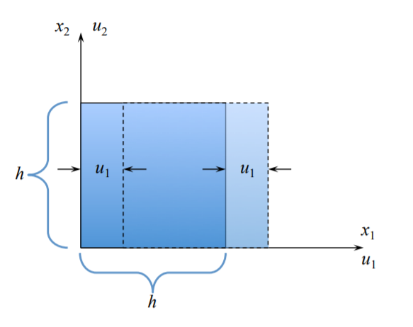
It follows from \ref{1.2.11} that the corresponding strain component vanishes, \(\epsilon_{11} = 0\). The first component of the spin tensor is zero from the definition, \(\omega_{11} = 0\).

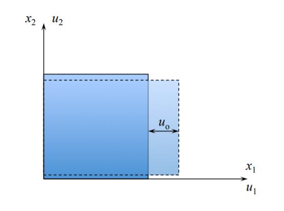
Extension along \(x_1\) axis

At \(x_1\): \(u_1 = 0\).

At \(x_1 + h\): \(u_1 = u_o\).

The corresponding strain is \(\epsilon_{11} = \frac{u_o}{h}\).

Pure shear on the \(x_1x_2\) plane

At \(x_1 = 0\) and \(x_2 = 0\): \(u_1 = u_2 = 0\)

At \(x_1 = h\) and \(x_2 = 0\): \(u_1 = 0\) and \(u_2 = u_o\)

At \(x_1 = 0\) and \(x_2 = h\): \(u_1 = u_o\) and \(u_2 = 0\)

Figure \(\PageIndex{2}\): The square element is stretched in one direction.

Figure \(\PageIndex{3}\): Imposing constant deformative gradients.

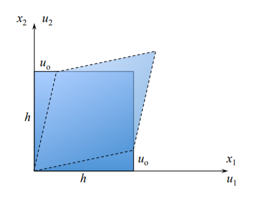
It follows from Equation \ref{1.2.10} and Equation \ref{1.2.6} that:

\[\epsilon_{12} = \frac{1}{2} \left( \frac{u_o}{h} +\frac{u_o}{h}\right) = \frac{u_o} {h}\]

\[\omega_{12} = \frac{1}{2} \left( \frac{u_o}{h} − \frac{u_o}{h}\right) = 0\]

The resulting strain is representing change of angles of the initial rectilinear element.

Rigid body rotation

At \(x_1 = 0\) and \(x_2 = 0\): \(u_1 = u_2 = 0\)

At \(x_1 = h\) and \(x_2 = 0\): \(u_1 = 0\) and \(u_2 = u_o\)

At \(x_1 = 0\) and \(x_2 = h\): \(u_1 = -u_o\) and \(u_2 = 0\)

Figure \(\PageIndex{4}\): An infinitesimal square element subjected to rigid body rotation.

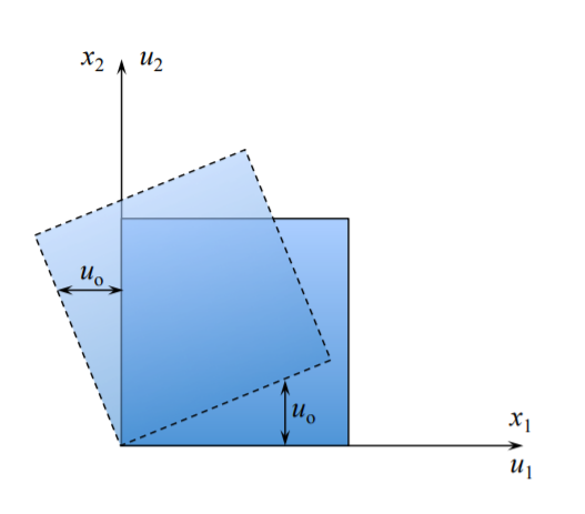
Changing the sign of \(u_1\) at \(x_1 = 0\) and \(x_2 = h\) from \(u_o\) to \(-u_o\) results in non-zero spin but zero strain

\[\epsilon_{12} = \frac{1}{2} \left( \frac{u_o}{h} + \left(− \frac{u_o}{h}\right)\right) = 0\]

\[\omega_{12} = \frac{1}{2} \left( \frac{u_o}{h} + \left(− \frac{u_o}{h}\right)\right) = \frac{u_o} {h}\]

The last example provides an explanation why the strain tensor was defined as a symmetric part of the displacement gradient. The physics dictates that rigid body translation and rotation should not induce any strains into the material element. In rigid body rotation displacement gradients are not zero. The strain tensor, defined as a symmetric part of the displacement gradient removes the effect of rotation in the state of strain in a body. In other words, strain described the change of length and angles while the spin, element rotation.