2.2: Advanced Topic - Local Equilibrium from the Principle of Virtual Work
- Page ID
- 21477

The derivation of the local equation of equilibrium from the global principle of virtual work is an elegant method in continuum and structural mechanics. This procedure also formulates static and kinematic boundary condition. There are two mathematical tools involved. One is the divergence theorem (Gauss-Green identity) and the other one is the concept of the calculus of variation.
The Gauss theorem transforms the volume integral into a surface integral
\[\int_{V} A_{i,i}dV = \int_{S} A_in_idS, \; A_{i,i} = \frac{\partial A_i}{\partial x_i} \label{2.2.1}\]
where \(A_i\) is a vector and ni is the unit normal vector of the surface element \(d\boldsymbol{S}\). In the simplest one-dimensional case, Equation \ref{2.2.1} is reduced to
\[\int_{x_1}^{x_2} \frac{dA}{dx} dx = A|_{x_1}^{x_2} = A(x_2) − A(x_1)\]
Starting from the definition of the infinitesimal strain given by Equation (2.1.22), the increments of the strain tensor and displacement vector are also linearly related
\[\delta \epsilon_{ij} = \frac{1}{2} (\delta u_{i,j} + \delta u_{j,i}) \label{2.2.3}\]
There is a fine difference between the symbol \(\delta u\) and \(du\), which is explained in Figure (\(\PageIndex{1}\)).
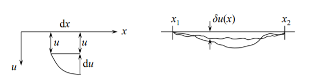
Both are linear operators and the rule for differentiations are the same.
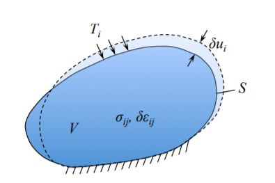
The principle of virtual work states that the incremental work of strains on the stresses over the volume of the body must be equal to the work of surface tractions in the incremental displacements over the surface of the body. Figure (\(\PageIndex{2}\)) helps to visualize the notation.
A part of the surface on which the displacement are zero \(\delta u_i = 0\) is denoted by \(S_\mathrm{U}\). The remainder of the surface \(S − S_\mathrm{U}\) is denoted by \(S_\mathrm{T}\). Mathematically the principle of virtual work states
\[\int_{V} \sigma_{ij}\delta \epsilon_{ij}dV = \int_{S} T_i\delta u_idS \label{2.2.4}\]
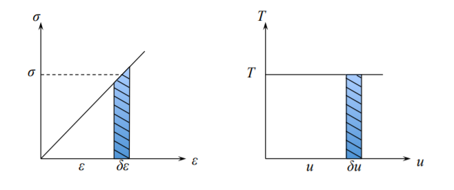
where \(\delta \epsilon_{ij}\) are calculated from \(\delta u_i\) using Equation \ref{2.2.3}. The one-dimensional graphical interpretation of the principle is shown in Figure (\(\PageIndex{3}\)).
The integrand of the left hand side of Equation \ref{2.2.4} can be transformed to a simpler form using the symmetry property of the stress tensor \(\sigma_{ij} = \sigma_{ji}\)
\[\frac{1}{2}\sigma_{ij} \delta u_{i,j} + \frac{1}{2}\sigma_{ji}\delta u_{j,i} = \sigma_{ij} \delta u_{i,j} \]
Recall an elementary rule of differentiation of the product of two functions
\[(ab)^{\prime} = a^{\prime} b + ab^{\prime}\]
which in application to our problem reads
\[\sigma_{ij} (\delta u_{i})_{,j} = (\sigma_{ij}\delta u_{i})_{,j} - (\sigma_{ij})_{,j} \delta u_{i} \label{2.2.7}\]
Now, the left hand side of Equation \ref{2.2.4} is transformed to
\[\int_{V} \sigma_{ij}\delta \epsilon_{ij}dV = \int_{V} \underbrace{(\sigma_{ij}\delta u_i)}_{A_i} \left._{,j} \right. dV - \int_{V} (\sigma_{ij})_{,j}\delta u_i dV \]
The first volume integral is now transformed to the surface integral according to Equation \ref{2.2.1}. Substituting this result into the statement of virtual work one gets
\[\int_{S} \sigma_{ij}\delta u_i n_j dS - \int_{V} \sigma_{ij,j}\delta u_i dV = \int_{S} T_i \delta u_i dS\]
Combining the two surface integrals into one integral we finally arrive at
\[\int_{S} (\sigma_{ij} n_i - T_i) \delta u_i dS - \int_{V} \sigma_{ij,j}\delta u_i dV = 0\]
The first integral vanishes when either
\[\sigma_{ij} n_i - T_i = 0 \text{ on } S_{\mathrm{T}}\]
\[\text{or } \delta u_i = 0 \text{ on } S_{\mathrm{U}}\]
The above equations represent respectively the stress and displacement boundary condition. The meaning of second integral should be interpreted in the spirit of the first lemma of the calculus of variation. The increment of the displacement vector \(\delta u_i\) can not vanish over the whole volume of the body because this would mean rigid body motion. The point is that the second integral in Equation \ref{2.2.7} must be zero not for one particular shape of \(\delta u_i\) but for all possible variation of the displacement field, as shown in Figure (\(\PageIndex{1}\)). Thus, the calculus of variation tell us that this is possible only when
\[\sigma_{ij,j} = 0 \text{ in } V \label{2.2.13}\]
The principle of virtual work is often called the weak (global) statement of equilibrium while Equation \ref{2.2.13} is the local equation of equilibrium but is not called strong. The weak statement of equilibrium is a starting point of developing most approximate methods in continuum and structural mechanics such as eigenvalue expansion, finite difference or finite element method. The critical assumption of the first lemma of the calculus of variation is that an infinity of different virtual velocities are considered. This is achieved by considering a large but finite degrees of freedom through many terms in the eigenvalue expansion or many discrete elements. Through this assumption the equivalence of the global and local formulation is achieved.
An alternative form of the principle of virtual work, extensively in plasticity theory is the principle of virtual velocity. By observing that
\[\delta u = \frac{du}{dt}\delta t = \dot{u} \delta t\]
Equation \ref{2.2.4} is transformed to
\[\int_{V} \sigma_{ij} \dot{\epsilon_{ij}} dV = \int_{S} T_i \dot{u_i} dS \]
where \(\dot{\epsilon_{ij}}\) is the instantaneous velocity field obtained from the incremental velocities \(\dot{u_i}\) through the linear geometric relation, Equation \ref{2.2.4}.
Generalized Stresses
This concept is introduced in order to reduce the two-dimensional problem in \(x\) and \(z\) in beams to one-dimensional problem in \(x\), governed by an ordinary differential equation.
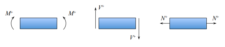
At an arbitrary cross-section in a beam one can distinguish a vector of bending moments \(\{M_x, M_y, T\}\) where \(M_x\) is bending the beam in the \((x, z)\) plane, \(M_y\) and \(T\) is the torque. (Do not confuse torque with surface traction vector). The meaning of the moment vector is explained in Figure (\(\PageIndex{4}\)).
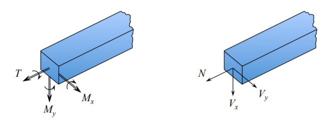
These are components of the bending moment vector. The components of the force vector acting at an arbitrary cross-section are \(\{V_x, V_y, N\}\) is the axial (membrane) force. In planar bending of a beam only three out of six components of the generalized stress resultants survival. They are defined by
\[M_x = M \buildrel \rm {def} \over{=} \int_{A} \sigma_{xx}z \, dA \; [\mathrm{Nm}]\]
\[N \buildrel \rm {def} \over{=} \int_{A} \sigma_{xx} \, dA \; [\mathrm{N}]\]
\[V_x = V \buildrel \rm {def} \over{=} \int_{A} \sigma_{\mathrm{xz}} \, dA \; [\mathrm{N}]\]
The product \(\sigma_{xx}{dA}\) in Equation (3.36a) is the incremental force. Multiplying this force by the “arm” \(z\) from the beam bending axis gives the incremental bounding moment \(dM = (\sigma_{xx}dA)z\). The total bending moment is an integral of \(dM\) over the beam cross-section. The sign of the generalized quantities is decided by the sign of the stress.
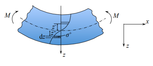
Imagine that the beam is bent in the way shown is Figure (\(\PageIndex{5}\)). On the tensile side of the beam the stress is positive, \(\sigma^+\) and so is the distance from the beam axis. On the compressive side both the stress and force arms are negative \(\sigma^-z^-\), but the product is positive. Therefore the tensile and compressive side of the beam contribute to the positive bending moment. The beam (or its portion) where the bending moment is negative is called the “smiling beam”. Therefore looking at the deformed shape of the beam one can determine immediately the sign of the bending moment. The sign of the axial and shear force can be easily determined from Figure (\(\PageIndex{6}\)).