
4.1: Governing Equations
- Page ID
- 21490

So far we have established three groups of equations fully characterizing the response of beams to different types of loading. In Chapter 1 relations were established to calculate strains from the displacement field.
\[\epsilon(x, z) = \epsilon^{\circ}(x) + z\kappa\]
where
\[\epsilon^{\circ}(x) = \frac{du}{dx} + \frac{1}{2} \left( \frac{dw}{dx} \right)^2 \; , \; \kappa = −\frac{d^2w}{dx^2} \label{4.1.2}\]
The above geometrical relation are independent on equilibrium and apply to any kind of materials.
The second set of equations, derived in Chapter 2, is the equilibrium requirement
\[\frac{dV^*}{dx} + q(x) = 0 \quad − \quad \text{ force equilibrium}\]
\[\frac{dM}{dx} - V = 0 \quad − \quad \text{ moment equilibrium} \label{4.1.4}\]
where \(V^* = V + N \frac{dw}{dx}\) is the effective shear.
\[\frac{dN}{dx} = 0 \]
Eliminating \(V\) and \(V^*\) between the above equations, the beam equilibrium equation was obtained (See Equation (2.7.1))
\[\frac{d^2M}{dx^2} + N\frac{d^2w}{dx^2} + q = 0 \label{4.1.7}\]
The derivation of the equilibrium is valid for all types of materials. In the theory of moderately large deflections, the equilibrium is coupled with the kinematics.
The third group of equation define the material behavior and relates the generalized strains to generalized forces
\[N = EA\epsilon^{\circ} \label{4.1.8}\]
\[M = EI\kappa \label{4.1.9}\]
Independence of geometry and equilibrium on constitutive equation allows to develop the general framework of a solver in the Finite Element codes. The constitutive equations can then be added as a user Defined Subroutines.
Let’s consider first the infinitesimal deformations (small rotations for which the term \(\frac{1}{2} \left( \frac{dw}{dx} \right)^2\) vanish in Equation \ref{4.1.2} and the term \(\frac{d^2w}{dx^2} = 0\) in Equation \ref{4.1.7}. Then from Equations \ref{4.1.2}, \ref{4.1.4} and \ref{4.1.8} one obtains
\[EA\frac{d^2u}{dx^2} = 0\]
Eliminating the curvature and bending moments between Equations \ref{4.1.2}, \ref{4.1.7} and \ref{4.1.9}, the beam deflection equation is obtained
\[EI\frac{d^4w}{dx^4} = q(x) \label{4.1.11}\]
The concentrated load \(P\) can be treated as a special case of the distributed load \(q(x) = P \delta(x − x_0)\), where \(\delta\) is the Dirac delta function.
Let’s consider first Equation \ref{4.1.4} for the axial displacement. The boundary conditions in the \(x\)-direction are
\[(N − \bar{N})\delta u = 0\]
The general solution for \(u(x)\) is
\[\frac{du}{dx} = D_1 \; , \; u = D_1x + D_0 \label{4.1.13}\]
There are two integration constants, and two boundary conditions are needed. There are only four combinations of boundary conditions:
1. Beam restricted from axial motion, see Figure (\(\PageIndex{1}\)).
\[u(x = 0) = u(x = l) = 0\]
This gives rise to the solution of two algebraic equation
\[0 = D_0 + D_1 \cdot 0\]
\[0 = D_0 + D_1l\]
which gives \(D_0 = D_1 = 0\) and \(u(x) = 0\). This is a trivial case, for which the axial force \(N = EA\frac{du}{dx}\) vanishes as well.
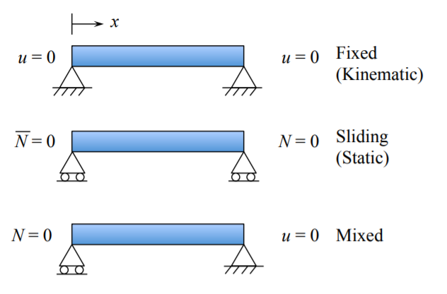
2. Beam allowed to slide in the \(x\)-direction on both ends.
\[\bar{N} = N = 0 \text{ at } x = 0 \text{ and } x = l\]
The axial force is proportional to \(\frac{du}{dx}\). From Equation \ref{4.1.13} we can see that the gradient of \(u\) is zero along the entire beam. So, if \(\bar{N} = 0\) or \(\frac{du}{dx}\) vanishes at one end, say \(x = 0\), \(D_1 = 0\) and automatically \(\bar{N} = 0\) is satisfied at the other end, \(x = l\). The integration constant \(D_0\) is undetermined meaning that the rigid body translation of the entire beam is allowed.
3. In order to prevent the rigid body translation, one end of the beam, say \(x = 0\), must be fixed against motion in the \(x\)-direction. Thus
\[\bar{N} = 0 \text{ or } \frac{du}{dx} = 0 \quad \text{ at } \quad x = 0\]
\[u = 0 \quad \text{ at } \quad x = l\]
which are precisely the boundary conditions for the third case. From Equation \ref{4.1.13} we get
\[D_1 = 0\]
\[D_1l + D_2 = 0 \rightarrow D_2 = 0 \]
Now, the axial displacement vanishes, \(u(x) = 0\) but the rigid body translation is eliminated.
For all the above three cases of kinematic static and mixed boundary conditions, the axial force was zero.
4. If one end of the beam (bar) is loaded by a given force \(\bar{N}\) and the other one is fixed, the boundary conditions (BC) are
\[\begin{array}{lcl} N = -\bar{N} \; , \; EA\frac{du}{dx} = 0 & \text{ at } x = 0 \\ u = 0 & \text{ at } x = l \end {array}\]
\[D_1 = − \frac{\bar{N}}{EA} \; , \; D_2 = \frac{\bar{N}l}{EA}\]
and the solution is
\[u(x) = \frac{\bar{N}}{EA} (l − x)\]
The case in which the nonlinear term is retained in Equation \ref{4.1.2} is much more interesting. This will be dealt with in the section on moderately large deflection of beams.
We now turn our attention to the solution of the beam deflection, Equation \ref{4.1.11}. This is the fourth-order linear inhomogeneous equation which requires four boundary conditions. There are four types of boundary conditions, defined by
\[(M − \bar{M})\delta w^{\prime} = 0\]
\[(V − \bar{V}) \delta w = 0\]
For the sake of illustration, we select a pin-pin BC for a beam loaded by the uniform like load \(q\), Figure (\(\PageIndex{2}\)).
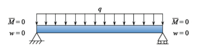
The bending moment is proportional to the curvature. Equation \ref{4.1.11} is then subjected to the following boundary conditions:
\[w(x = 0) = w(x = l) = 0\]
\[\left. \frac{d^2w}{dx^2}\right|_{x=0} = \left. \frac{d^2w}{dx^2} \right|_{x=l} = 0 \]
Let’s integrate the differential equation four times with respect to \(x\):
\[\begin{align} \frac{d^3w}{dx^3} &= \frac{qx}{EA} + C_1 \\[4pt] \frac{d^2w}{dx^2} &= \frac{qx^2}{EA2} + C_1x + C_2 \\[4pt] \frac{dw}{dx} &= \frac{qx^3}{EA6} + \frac{C_1x^2}{2} + C_2x + C_3 \\[4pt] w &= \frac{qx^4}{EA24} + \frac{C_1x^3}{6} + \frac{C_2x^2}{2} + C_3x + C_4 \end{align}\]
Substituting the BC into the general solutions, one gets
\[0 = C_2\]
\[0 = \frac{ql^3}{2EA} + {C_1}l + C_2 \]
\[0 = C_4\]
\[0 = \frac{ql^4}{24EA} + \frac{C_1l^3}{6} + \frac{C_2l^2}{2} + C_3l + C_4 \]
The solution of the above system is
\[C_1 = −\frac{ql}{2}\]
\[C_2 = 0\]
\[C_3 = \frac{ql^3}{12}\]
\[C_4 = 0\]
The load-displacement relation becomes
\[w(x) = \frac{qx}{24EA}(l^3 - 2lx^2 + x^3) \label{4.1.40}\]
Differentiating Equation \ref{4.1.40} twice, the expression for the bending moment is
\[M(x) = \frac{qx}{2} (l − x)\]
and differentiating again, the shear force becomes
\[V(x) = \frac{dM}{dx} = \frac{q}{2} (l − 2x)\]
Plots of the normalized bending moments and shear forces are shown in Figure (\(\PageIndex{3}\)).
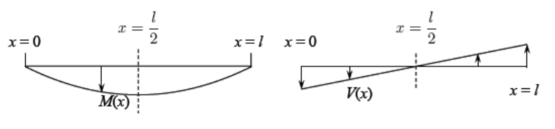
The shear force \(V = EI\frac{d^3w}{dx^3}\) is seen to vanish at the mid-span of the beam. Also the slope \(\frac{dw}{dx}\) is zero at this location. We have proved that at the symmetry plane
\[V (x = \frac{l}{2} ) = 0 \label{4.1.43}\]
\[\left. \frac{dw}{dx}\right|_{x= \frac{l}{2}} = 0 \label{4.1.44}\]
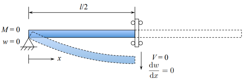
Inversely, if the problem is symmetric, that Equations \ref{4.1.43}-\ref{4.1.44} must hold at the symmetry plane. As an alternative formulation, one can consider a half of the beam with the symmetry BC.
Can you solve the above problem and compare it with solution of the pin-pin beam, Equation \ref{4.1.40}?
It should be mentioned that the pin-pin supported beam is a statically determinate structure. Therefore the distribution of shear forces and bending moments can be determined from the equilibrium equation alone. Can you do it and get correctly the signs?
The purpose of Chapter 4 is to present properties of the governing equations and solutions. interested students are referred to end chapter of problem sets where many beams with different loading and BC are considered. Also the recommended reference book and monographs present solution to some common beam problems.