
9.3: Snap-through of a Two Bar System
- Page ID
- 21527

This is a very interesting problem, because it summaries and even extends our knowledge.
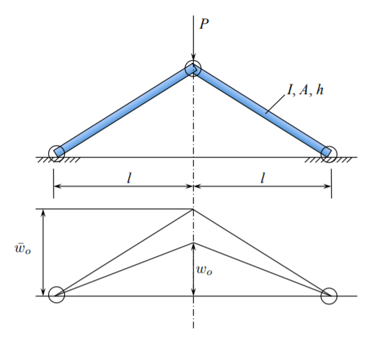
There are three hinges so that each rod is a pin-pin column. The rods are elastic characterized by the bending rigidity \(EI\), axial rigidity \(EA\). The initial stress-free configuration is defined by the height \(\bar{w}_o\), which was previously called the amplitude of initial imperfection.
Here, \(\bar{w}_o\) should be regarded as the initial shape of the structure. Upon application of the load, a compressive axial force develops in the rod, their length shortens allowing for a straight (flat) configuration. The system snaps into a new configuration where tensile force develops in the rods. Depending on the slenderness ratio, they may buckle sometime during the loading process.
Pre-buckling solution
Due to the unmovable hinges, the in-plane components of the displacement is zero, \(u = 0\). The strain in the bars develops by the presence of finite rotations
\[\epsilon = \frac{1}{2} (w^{\prime})^2 − \frac{1}{2}(\bar{w}^{\prime})^2 \label{10.33}\]
In the pre buckling configuration the rods are straight, so
\[w^{\prime} = \frac{w_o}{l}, \quad \bar{w}^{\prime} = \frac{\bar{w}_o}{l} \]
and Equation \ref{10.33} reduces to
\[\epsilon = \frac{1}{2} \left(\frac{w_o}{l}\right)^2 − \frac{1}{2} \left(\frac{\bar{w}_o}{l}\right)^2 \]
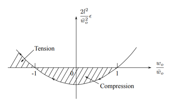
The plot of the dimensionless strain versus the ratio \(w_o/\bar{w}_o\) is shown in Figure (\(\PageIndex{3}\)). From the elasticity law, the axial force in the rod is
\[N = EA \epsilon = \frac{EA}{2} \left[ \left(\frac{w_o}{l}\right)^2 − \left(\frac{\bar{w}_o}{l}\right)^2 \right] = \begin{cases} \text{compressive for } − w_0 \leqslant w_o \leqslant \bar{w}_o \\ \text{tensile for } w_o < −\bar{w}_o \end{cases} \label{10.36}\]
Equilibrium between the external load \(P\) and the membrane force \(N\) requires that
\[P = −2N \frac{w_o}{l} \label{10.37}\]
Eliminating the force \(N\) between Equations \ref{10.36} and \ref{10.37} yields
\[− \frac{P}{2}\frac{l}{w_o} = EA \left[ \frac{1}{2} \left(\frac{w_o}{l}\right)^2 − \frac{1}{2} \left(\frac{\bar{w}_o}{l}\right)^2 \right]\]
or in a dimensionless form
\[\bar{P} = \delta(\bar{\delta}^2 − \delta^2) \label{10.39}\]
where
\[\bar{P} = \frac{P}{EA}, \quad \delta = \frac{w_o}{l}, \quad \bar{\delta} = \frac{\bar{w}_o}{l} \]
The equilibrium path given by Equation \ref{10.39} is the third order parabola with three roots at \(\delta = 0, \delta = \pm \bar{\delta}\), see Figure (\(\PageIndex{4}\)).
The loading process starts at A and the portion of the trajectory AB is stable. The point B is the instability point. In the process is force controlled, there is a jump to the next equilibrium configuration which is point E. So the system “snaps” into a tensile configuration and this transition is in reality a dynamic problem. The process can be displacement control and then the force \(\bar{P}\) is the reaction force which is positive on the segments ABC and EF but negative on the segment CDE of the trajectory. This means that an opposite force \(\bar{P}\) is required on CDE to keep the system in static equilibrium. By contrast, in the force controlled process the inertia force is equilibrating the system at any time. The maximum force occurs when
\[\frac{dP}{d\delta} = \bar{\delta}^2 − 3\delta^2 = 0 \]
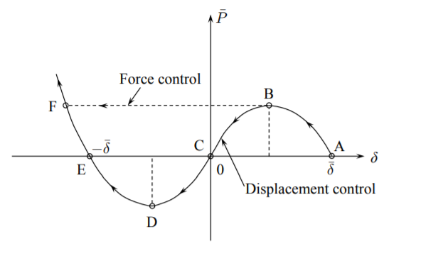
The maximum occurs at \(\delta = \bar{\delta}/\sqrt{3}\) and the maximum force is \(\bar{P}_{\text{max}} = \frac{2}{3 \sqrt{3}} \bar{\delta}^3\).
Any time during the loading phase AB there is a possibility for the rods to buckle. The instant of buckling is detected by equating the axial force from Equation (10.37) to the critical buckling force of the pin-pin column
\[N = \frac{P_{cr}}{2}\frac{l}{w_o} = \frac{\pi^2 EI}{l^2} \label{10.42}\]
The dimensionless version of this equation is
\[\bar{P}_{cr} = \frac{P_{cr}}{EA} = 2\pi^2 \frac{\delta}{\beta^2} \]
where \(\beta = \frac{l}{r}\) is the slenderness ratio, and \(r^2 = \frac{I}{A}\) is the radius of gyration of the crosssection. In the coordinate system \((\bar{P}, \delta)\), the buckling point is determined by the intersection of the straight line, Equation \ref{10.42}, and the third order parabola
\[\frac{2\pi^2}{\beta^2}\delta = \delta(\bar{\delta}^2 − \delta^2_c ) \]
The displacement to buckle is
\[\delta_c = \sqrt{\bar{\delta}^2 − \frac{2\pi^2}{\beta^2}} \]
and the corresponding buckling force \(\bar{P}_c\) is
\[\bar{P}_c = \frac{2\pi^2}{\beta^2} \sqrt{ \bar{\delta}^2 − \frac{2\pi^2}{\beta^2}} \]
The graphical interpretation of the above analysis is shown in Figure (\(\PageIndex{5}\)).
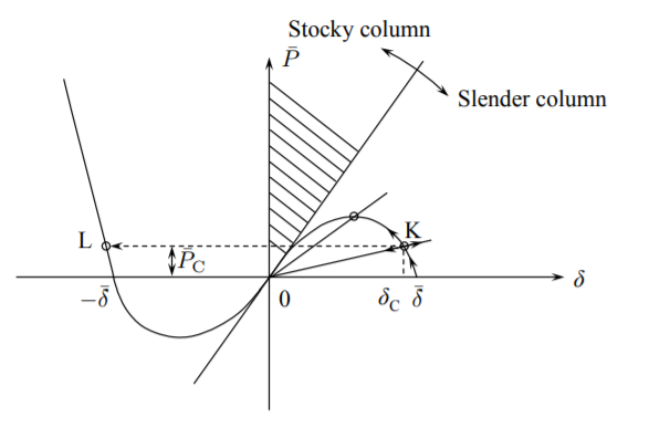
There is a family of straight lines with the slenderness ratio as a parameter. The critical slenderness ratio for which buckling will never occur is
\[\beta^2_{cr} = \frac{2\pi}{\bar{\delta}} \]
This situation corresponds to the straight line tangent to the third order parabola. Of practical interest is the situation in which the bifurcation point occurs before the maximum force is reached at \(\delta_{\text{max}} = \bar{\delta}/\sqrt{3}\) and \(\bar{P}_{\text{max}} = \frac{2}{3 \sqrt{3}}\bar{\delta}^3\). The corresponding minimum slenderness ratio, calculated from Equation \ref{10.42} is
\[\beta_{\text{min}}^2 = \frac{\sqrt{3} \pi}{\bar{\delta}} \]
To sum up, there are three ranges of the slenderness ratio:
| \(\beta_{\text{min}} < \beta < \infty\) | \(\beta = \beta_{\text{min}}\) | \(\beta = \beta_{\text{min}}\) | |
|---|---|---|---|
| \(\bar{P}_{\text{max}}\) | \(\frac{2}{3\sqrt{3}}\bar{\delta}^3\) | No buckling static or dynamic equilibrium path | |
| \(\delta_{\text{max}}\) | \(\frac{\bar{\delta}}{\sqrt{3}}\) | No buckling static or dynamic equilibrium path |
For the square cross-section \(h \times h\), the critical combination of the geometrical parameters
\[\frac{\bar{w}_o}{h} = 36 \pi \frac{h}{l}\]
From the above solution, we conclude that snap-through of the bar system without buckling will occur only for very shallow systems.