10.5: Post-buckling Response of Plates (Advanced)

Let’s assumed that the plate is subjected to a monotonically increasing axial compression \(u_o\), Figure (\(\PageIndex{1}\)).

Figure \(\PageIndex{1}\): Two degree-of-freedom model of the buckled plate.

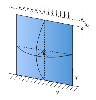
Initially the plate is straight and in the pre-buckling state there is uniaxial compression and bi-axial deformation. This stage was analyzed in Section 6.1. there was no out-of-plane displacement \(w_o\). The bifurcation point was tested by imposing an arbitrary small field of out-of-plane displacement. Now, some of the compression energy is relieved, but the bending energy appears so that the total potential energy of the system remains the same.

The corresponding value of the load (buckling load) under which this happens was derived in Section 6.2. What happens to the plate after buckling has occurred is the subject of the present section. The deformation of the plate is assumed to be a superposition of the in-plane compression. The form of the in-plane displacement is similar as in the prebuckling solution, Equation (??), but now one more term should be added to the expression for \(u_y\) in order to satisfy zero traction at the unloaded edges.

\[u_x = u_o \left( 1 − \frac{x}{a}\right)\]

\[u_y = \nu u_o \frac{y}{a} + f(x) \]

The field of out-of-plane deformation is taken identical as in the buckling solution

\[w = w_o \sin \frac{\pi x}{a} \sin \frac{\pi y}{b}\]

which satisfies the simply supported boundary conditions at all four edges. Here it is assumed that the plate is either infinitely long or is square so that \(a = b\).

The total potential energy of the system is

\[\prod = U_b + U_m − P U_o \]

where \(P = bN\) and expression for the bending and membrane energies are given by Equations (3.6.25) and (3.6.41), respectively. The curvature tensor is defined by

\[\kappa_{\alpha\beta} = −w_{,\alpha\beta} \]

and for the assumed shape \(w(x, y)\) has three components

\[\kappa_{\alpha\beta} = w_o \left(\frac{\pi}{a}\right)^2 \begin{vmatrix} \sin \frac{\pi x}{a} \sin \frac{\pi y}{a} & - \cos \frac{\pi x}{a} \cos \frac{\pi y}{a} \\ - \cos \frac{\pi x}{a} \sin \frac{\pi y} {a} & \sin \frac{\pi x}{a} \sin \frac{\pi y}{a} \end{vmatrix}\]

The membrane strain results from the gradient of in-plane displacement vector and the moderately large rotation of plate elements

\[\epsilon_{\alpha\beta} = \frac{1}{2} (u_{\alpha,\beta} + u_{\beta,\alpha}) + \frac{1}{2} w_{,\alpha} w_{,\beta} \]

The components of the in-plane strain tensors are

\[\left.\begin{array}{l} \epsilon_{xx} = − \frac{u_o}{a} + \frac{w^2_o}{2} \left(\frac{\pi}{a}\right)^2 \cos^2 \frac{\pi x}{a} \sin^2 \frac{\pi y}{a} \\ \epsilon_{yy} = \nu\frac{u_o}{a} + f^{\prime}(x) + \frac{w^2_o}{2} \left(\frac{\pi}{a}\right)^2 \sin^2 \frac{\pi x}{a} \cos^2 \frac{\pi y}{a} \end{array}\right\} \]

\[\epsilon_{xy} = \frac{w^2_o}{2} \left( \frac{\pi}{a}\right)^2 \cos^2 \frac{\pi x}{a} \cos^2 \frac{\pi y}{a} \]

It is seen that the form of the axial strain \(\epsilon_{xx}\) provides coupling between the in-plane amplitude \(u_o\) and the out-of-plane amplitude \(w_o\).

The general expression for the bending energy of the plate, Equation (3.6.25) is

\[U_b = \frac{D}{2} \int^{a}_{0} \int^{a}_{0} \{(\kappa_{xx} + \kappa_{yy})^2 − 2(1 − \nu)\kappa_G\} dx dy \]

where \(\kappa_G = \kappa_{xx}\kappa_{yy} − \kappa^2_{xy}\) is the Gaussian curvature. It can be easily shown that the Gaussian curvature integrated over the surface of the plate is zero. Therefore, the second term in the integrand of Equation (10.3.1) vanishes. Finally, the total bending energy of the plate is calculated to be

\[U_b = \frac{1}{2} Dw^2_o \frac{\pi^4}{a^2} \]

Before proceeding to calculate the membrane strain energy, the unknown function \(f(x)\) in Equation (??) should be determined from the boundary condition \(N_{yy}(y = a \text{ and } y = 0) = 0\). The plane stress elasticity law is

\[N_{xx} = C(\epsilon_{xx} + \nu \epsilon_{yy}) \]

\[N_{yy} = C(\epsilon_{yy} + \nu \epsilon_{xx}) \]

\[N_{xy} = (1 - \nu) C \epsilon_{xy} \]

From Equation (10.2.10-10.2.11), the in-plane membrane force in the y-direction is

\[N_{yy} =C \left[ \nu \frac{u_o}{a} + \frac{1}{2} w^2_o \left(\frac{\pi}{a}\right)^2 \sin^2 \frac{\pi x}{a} \cos^2 \frac{\pi y}{a} + f^{\prime} \\ −\nu \frac{u_o}{a} + \frac{\nu}{2} w^2_o \left(\frac{\pi}{a}\right)^2 \cos^2 \frac{\pi x}{a} \sin^2 \frac{\pi y}{a} \right] \]

The membrane force changes from point to point and at the unloaded edges \(y = 0\) and \(y = a\) is

\[N_{yy} (0, a) = C \left[ \frac{1}{2} w^2_o \left(\frac{\pi}{a}\right)^2 \ sin^2 \frac{\pi x}{a} + f^{\prime} \right] \]

Now, the total membrane energy of the plate can be calculated. After lengthy algebra, the final expression is

\[U_m = \frac{C}{2} \left[ (1 − \nu^2 )u^2_o − 2(1 − \nu^2 ) \frac{\pi^2}{8} \frac{u_o}{a} w^2_o + (3 − 2\nu) \frac{\pi^4}{64} \frac{w^4_o}{a^2} \right] \]

The total potential energy of the system is

\[\prod (u_o, w_o) = U_b + U_m − P u_o \]

The equilibrium of the system requires that the first variation of the total potential energy vanishes \(\delta \prod (u_o, w_o) = 0\). This leads to two equations

\[\frac{\partial \prod}{\partial u_o} = 0 \rightarrow P = (1 − \nu^2 )C \left[ u_o − \frac{\pi^2}{8}\frac{w^2_o}{a}\right] \]

\[\frac{\partial \prod}{\partial w_o} = 0 \rightarrow 64 \left(\frac{\pi}{a}\right)^2 w_o \left[ \frac{4 \pi^2 D}{C} − (1 − \nu^2 )au_o + (3 − 2\nu) \frac{\pi^2}{8} w^2_o \right] = 0 \]

There are two solutions of the above system. The pre-buckling solution is recovered by setting \(w_o = 0\). Then from Equation (??)

\[P = (1 − \nu^2 )Cu_o = (1 − \nu^2 ) \frac{Eh}{1 − \nu^2} u_o = Ehu_o \label{11.44}\]

and Equation (??) is satisfied identically. The solution (??) is exact and is equal to the one derived in Section 10.1 of Chapter 10. In the post-buckling range \(w_o > 0\) and Equation (??) provides a unique relation between the in-plane and out-of-plane amplitude of the assumed displacement field

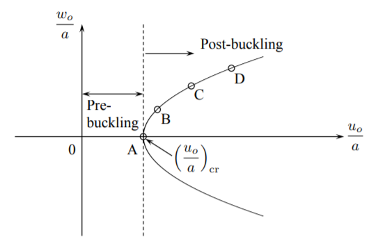
\[\frac{\pi^2}{8}\left(\frac{w_o}{a}\right)^2 = \frac{1 - \nu^2}{3 - 2\nu} \frac{u_o}{a} - \frac{4 D \pi^2}{C(3-2\nu) a^2} \]

The plot of the function \(w_o = w_o(u_o)\) is shown in Figure (\(\PageIndex{2}\)).

The critical displacement \((u_o)_c\) to buckle, corresponding to the point of buckling, is obtained from Equation (??) by setting \(w_o = 0\)

\[(u_o)_c = \frac{4\pi^2D}{a} \frac{1}{C(1 − \nu^2)} \]

Figure \(\PageIndex{2}\): The out-of-plane displacement amplitude.

Eliminating \(w_o\) between Equations (??) and (??) gives a linear post-buckling solution

\[P = \frac{13}{25} (1 − \nu^2 )Cu_o + \frac{1 − \nu^2}{3 − 2\nu}\frac{4\pi^2 D}{a} \]

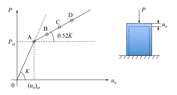
The post-buckling stiffness \(K_{\text{post}} = \frac{dD}{du_o}\) is

\[K_{\text{post}} = \frac{13}{25} (1 − \nu^2)C = 0.52K_{\text{pre}}\]

where \(K_{\text{pre}}\) is the pre-buckling stiffness. For all practical purposes it can be assumed that the plate is loosing half of its stiffness after buckling but is able to carry additional loads. Based on the above analysis, the load-displacement relation of an elastic plate is depicted in Figure (\(\PageIndex{3}\)).

Figure \(\PageIndex{3}\): Pre and post-buckling response of a plate.

Substituting the expression for \((u_o)_c\) into Equation \ref{11.44}, the predicted buckling load is

\[P_c = \frac{4\pi^2D}{a}\]

which is the exact solution of the problem.