2.1: Types of Structural Loads

Dead Loads

Dead loads are structural loads of a constant magnitude over time. They include the self-weight of structural members, such as walls, plasters, ceilings, floors, beams, columns, and roofs. Dead loads also include the loads of fixtures that are permanently attached to the structure. Prior to the analysis and design of structures, members are preliminarily sized based on architectural drawings and other relevant documents, and their weights are determined using the information available in most codes and other civil engineering literature. The recommended weight values of some commonly used materials for structural members are presented in Table 2.1. The determination of the dead load due to structural members is an iterative process. During design, member sizes and weight could change, and the process is repeated until a final member size is obtained that could support the member’s weight and the superimposed loads.

Table 2.1: Unit weights of construction materials.

Material	Unit Weight
	lb/ft^3	kN/m^3
Reinforced concrete Plain concrete Structural steel Aluminum Brick Concrete masonry unit Wood (Douglas fir larch) Engineered wood (plywood)	150 145 490 165 120 135 34 36
		23.60 22.60 77.00 25.90 18.90 21.20 5.30 5.7

Example \(\PageIndex{1}\)

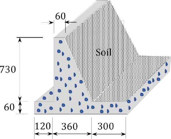
The semi-gravity retaining wall shown in Figure 2.1 Figure 2.1 is made of mass concrete with a unit weight of 23.6 \(\mathrm{kN} / \mathrm{m}^{3}\). Determine the length of the wall’s weight per foot.

Solution

\(\text { Area of wall }=(7.8 \mathrm{m})(0.6 \mathrm{m})+(7.3 \mathrm{m})(0.6 \mathrm{m})+\left(\frac{1}{2}\right)(3 \mathrm{m})(7.3 \mathrm{m})=20.01 \mathrm{m}^{2}\)

\(\text { Length of the wall's weight per foot }=20.01 \mathrm{m}^{2} \times\left(23.6 \mathrm{kN} / \mathrm{m}^{3}\right)=472.24 \mathrm{kN} / \mathrm{m}\)

Live Loads

 

Table 2.2: Minimum uniform and concentrated floor live loads.

Occupancy or Use	Live Load
	Uniform psf (kN/m^2)	Concentrated lb (kN)
Residential dwellings, apartments, hotels Private rooms and corridors serving them Public rooms and corridors serving them	40 (1.92) 100 (4.79)
Hospitals Patient rooms Operating rooms, laboratories Corridors above first floor	40 (1.92) 60 (2.87) 80 (3.83)	1,000 (4.45) 1,000 (4.45) 1,000 (4.45)
Office buildings Lobbies and first floor corridors Offices Corridors above first floor	100 (4.79) 50 (2.40) 80 (3.83)	2,000 (8.90) 2,000 (8.90) 2,000 (8.90)
Recreational Uses Bowling alleys, poolrooms, and similar uses Dance halls and ballrooms, gymnasiums Stadiums and arenas with fixed seats	75 (3.59) 100 (4.79) 60 (2.87)
Stores Retail First floor Upper floors Wholesale, all floors	100 (4.79) 75 (3.59) 125 (6.00)	1,000 (4.45) 1,000 (4.45) 1,000 (4.45)
Storage, warehouses Light Heavy	125 (6.00) 250 (11.97)
Manufacturing Light Heavy	125 (6.00) 250 (11.97)	2,000 (8.90) 3,000 (13.40)
Schools Classrooms Corridors above first floor First floor corridors	40 (1.92) 80 (3.83) 100 (4.79)	1,000 (4.45) 1,000 (4.45) 1,000 (4.45)

 

Example \(\PageIndex{1}\)

The floor system of the classroom shown in Figure 2.2 consists of a 3-inch-thick reinforced concrete slab supported by steel beams. If the weight of each steel beam is 62 \(\mathrm{lb} / \mathrm{ft}\), determine the dead load in \(\mathrm{lb} / \mathrm{ft}\) supported by any interior beam.

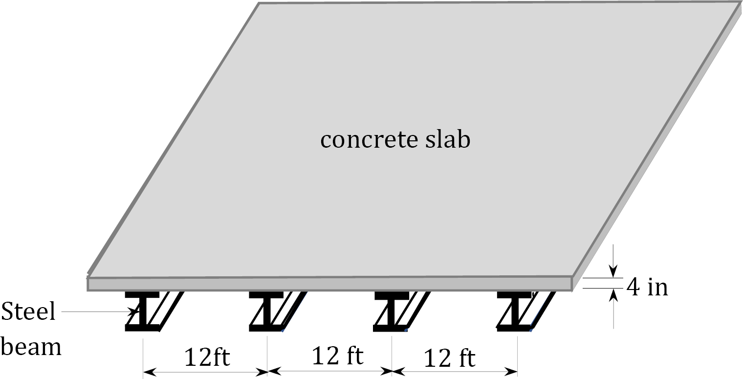
\(Fig. 2.2\). Classroom floor system.

Solution

Dead load due to slab weight \(=(12 \mathrm{ft})\left(\frac{4 \mathrm{in}}{12}\right)\left(150 \mathrm{lb} / \mathrm{ft}^{3}\right)=600 \mathrm{lb} / \mathrm{ft}\)

Dead load due to beam weight\(=62 \mathrm{lb} / \mathrm{ft}\)

Live load due to occupancy or use (classroom) \(=\left(40 \mathrm{lb} / \mathrm{ft}^{2}\right)(12 \mathrm{ft})=480 \mathrm{lb} / \mathrm{ft}\)

Total uniform load on steel beam \(=1142 \mathrm{lb} / \mathrm{ft}=1.142 \mathrm{k} / \mathrm{ft}\)

Impact Loads

Impact loads are sudden or rapid loads applied on a structure over a relatively short period of time compared with other structural loads. They cause larger stresses in structural members than those produced by gradually applied loads of the same magnitude. Examples of impact loads are loads from moving vehicles, vibrating machinery, or dropped weights. In practice, impact loads are considered equal to imposed loads that are incremented by some percentage, called the impact factor. Some building load impact factors are presented in Table 2.3. The American Association of State Highway and Transportation Officials (AASHTO) specifies the following expression for the computation of the impact factor for a moving truck load for use in highway bridge design:

\(\begin{aligned}
&I=\frac{50}{L+125} \leq 0.3 \quad \text { U.S. customary units }\\
&I=\frac{15.2}{L+38.1} \leq 0.3 \text { SI units }
\end{aligned}\)

where

\(I\) = impact factor.

= length in feet (or meters) of the span-loaded segment to cause maximum stress in the member under consideration.

Table 2.3: Building live load impact factors, as specified in ASCE/SEI 7-16.

Loading Case	I(%)
Elevator supports and machinery Light machinery supports Reciprocating machine supports Hangers supporting floors and balconies Crane support girders and their connections	100 20 50 33 25

Environmental Loads

2.1.4.1 Rain Loads

 

\(\begin{aligned}
&R=5.2\left(d_{s}+d_{h}\right) \quad \text { U.S. customary unit }\\
&R=0.0098\left(d_{s}+d_{h}\right) \text { SI units }
\end{aligned}\)

where

\(R\) = rain load on the undeflected roof, in psi or \(\mathrm{KN} / \mathrm{m}^{2}).

\(d_{S}\) = depth of water on the undeflected roof up to the inlet of the secondary drainage system (i.e. the static head), in inches or mm.

\(d_{h}\) = additional depth of water on the undeflected roof above the inlet of the secondary drainage system (i.e. the hydraulic head), in inches or mm. It depends on the flow rate, the size of the drainage, and the area drained by each drain.

The flow rate, \(Q\), in gallons per minute, can be computed as follows:

\(Q(\mathrm{gpm})=0.0104 Ai\)

where

\(A\) = roof area in square feet drained by the drainage system.

\(i\) = 100-yr., 1-hr. rainfall intensity in inches per hour for the building location specified in the plumbing code.

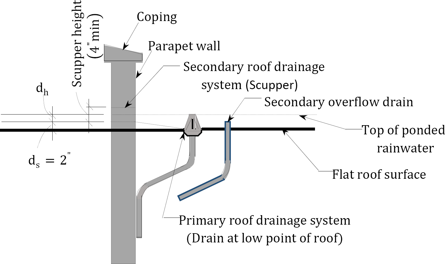
\(Fig. 2.3\). Roof drainage system (Adapted from the International Code Council).

2.1.4.2 Wind Loads

Wind loads are pressures exacted on structures by wind flow. Wind forces have been the cause of many structural failures in history, especially in coastal regions. The speed and direction of wind flow varies continuously, making it difficult to predict the exact pressure applied by wind on existing structures. This explains the reason for the considerable research efforts on the effect and estimation of wind forces. Figure 2.4 shows a typical wind load distribution on a structure. Based on Bernoulli’s principle, the relationship between dynamic wind pressure and wind velocity can be expressed as follows when visualizing the flow of wind as that of a fluid: \[q=\frac{1}{2} \rho V^{2}\]

where

\(q\) = dynamic wind pressure air in pounds per square foot.

\(\rho\) = mass density of air.

\(V\) = wind velocity in miles per hour.

Basic wind speed for specific locations in the continental United States can be obtained from the basic speed contour map in ASCE 7-16.

Assuming that the unit weight of air for a standard atmosphere is 0.07651 lb/ft³ and substituting this value into the previously stated equation 2.1, the following equation can be used for static wind pressure: \[q=\left(\frac{0.0765}{32.2}\right)\left(\frac{5280}{3600}\right)^{2} \frac{V^{2}}{2}=0.00256 V^{2}\]

To determine the magnitude of wind velocity and its pressure at various elevations above ground level, the ASCE 7-16 modified equation 2.2 by introducing some factors to account for the height of the structure above ground level, the importance of the structure in regard to human life and property, and the topography of its location, as follows: \[\begin{array}{ll}
q_{z}=0.00256 K_{z} K_{z t} K_{d} K_{e} V^{2} & \text { Customary units (lb/ft }^{2} \text { ) } \\
q_{z}=0.613 K_{z} K_{z t} K_{d} K_{e} V^{2} & \text { SI units }\left(\mathrm{N} / \mathrm{m}^{2}\right)
\end{array}\]

where

\(K_{Z}\) = the velocity pressure coefficient that depends on the height of the structure and the exposure condition. The values of \(K_{Z}\) are listed in Table 2.4.

\(K_{z t}\) = a topographic factor that accounts for an increase in wind velocity due to sudden changes in topography where there are hills and escarpments. This factor is an equal unity for building on level ground and increases with elevation.

\(K_{d}\) = wind directionality factor. It accounts for the reduced probability of maximum wind coming from any given direction and for the reduced probability of the maximum pressure developing on any wind direction most unfavorable to the structure. For structures subjected to wind loads only, \(K_{d} = 1\); for structures subjected to other loads, in addition to a wind load, \(K_{d}\) values are tabulated in Table 2.5.

\(K_{e}\) = ground elevation factor. According to section 26.9 in ASCE 7-16, it is expressed as \(K_{e} = 1\) for all elevations.

\(V\) = velocity of wind measured at a height z above ground level.

The three exposure conditions categorized as B, C, and D in Table 2.4 are defined in terms of surface roughness, as follows:

Exposure B: The surface roughness for this category includes urban and suburban areas, wooden areas, or other terrain with closely spaced obstructions. This category applies to buildings with mean roof heights of \(\leq\) 30 ft (9.1 m) if the surface extends in the upwind direction for a distance greater than 1,500 ft. For buildings with mean roof heights greater than 30 ft (9.1 m), this category will apply if the surface roughness in the upwind direction is greater than 2,600 ft (792 m) or 20 times the height of the building, whichever is greater.

Exposure C: Exposure C applies where surface roughness C prevails. Surface roughness C includes open terrain with scattered obstructions having heights less than 30 ft.

Exposure D: The surface roughness for this category includes flats, smooth mud flats, salt flats, unbroken ice, unobstructed areas, and water surfaces. Exposure D applies where surface roughness D extends in the upwind direction for a distance greater than 5,000 ft or 20 times the building height, whichever is greater. This also applies if the surface roughness upwind is B or C, and the site is within 600 ft (183 m) or 20 times the building height, whichever is greater.

Table 2.4: Velocity pressure exposure coefficient, K_z, as specified in ASCE 7-16.

Height z above ground level ft (m)	Kz
	Exposure
	B	C	D
0-15 (0-4.6)	0.57 (0.70)*	0.85	1.03
20 (6.1)	0.62 (0.70)	0.90	1.08
25 (7.6)	0.66 (0.70)	0.94	1.12
30 (9.1)	0.70	0.98	1.16
40 (12.2)	0.76	1.04	1.22
50 (15.2)	0.81	1.09	1.27
60 (18.0)	0.85	1.13	1.31
70 (21.3)	0.89	1.17	1.34
80 (24.4)	0.93	1.21	1.38
90 (27.4)	0.96	1.24	1.48

Table 2.5. Wind directional factor, K_d, as specified in ASCE 7-16.

Structure Type	Kd
Main wind force resisting system (MWFRS) Components and cladding	0.85 0.85
Arched roofs	0.85
Chimneys, tanks, and similar structures Square Hexagonal Round	0.9 0.95 0.95
Solid freestanding walls and solid freestanding and attached signs	0.85
Open signs and lattice framework	0.85
Trussed towers Triangular, square, rectangular All other cross sections	0.85 0.95

To obtain the final external pressures for the design of structures, equation 2.3 is further modified, as follows: \[P_{z}=q_{z} G C_{p}\]

where

\(P_{z}\) = design wind pressure on a face of the structure at height \(z\) above ground level. It increases with the height on the windward wall, but it is constant with the height on the leeward and side walls.

\(G\) = gust effect factor. \(G\) = 0.85 for rigid structures with a natural frequency of \(\geq\) 1 Hz. The gust factors for flexible structures are calculated using the equations in ASCE 7-16.

\(C_{p}\) = external pressure coefficient. It is a fraction of the external pressure on the windward walls, leeward walls, side walls, and roof. The values of C_p are presented in Tables 2.6 and 2.7.

To compute the wind load that will be used for member design, combine the external and internal wind pressures, as follows: \[P=q_{z} G C_{p}-q_{h}\left(G C_{p i}\right)\]

where

\(G C_{p i}\) = the internal pressure coefficient from ASCE 7-16.

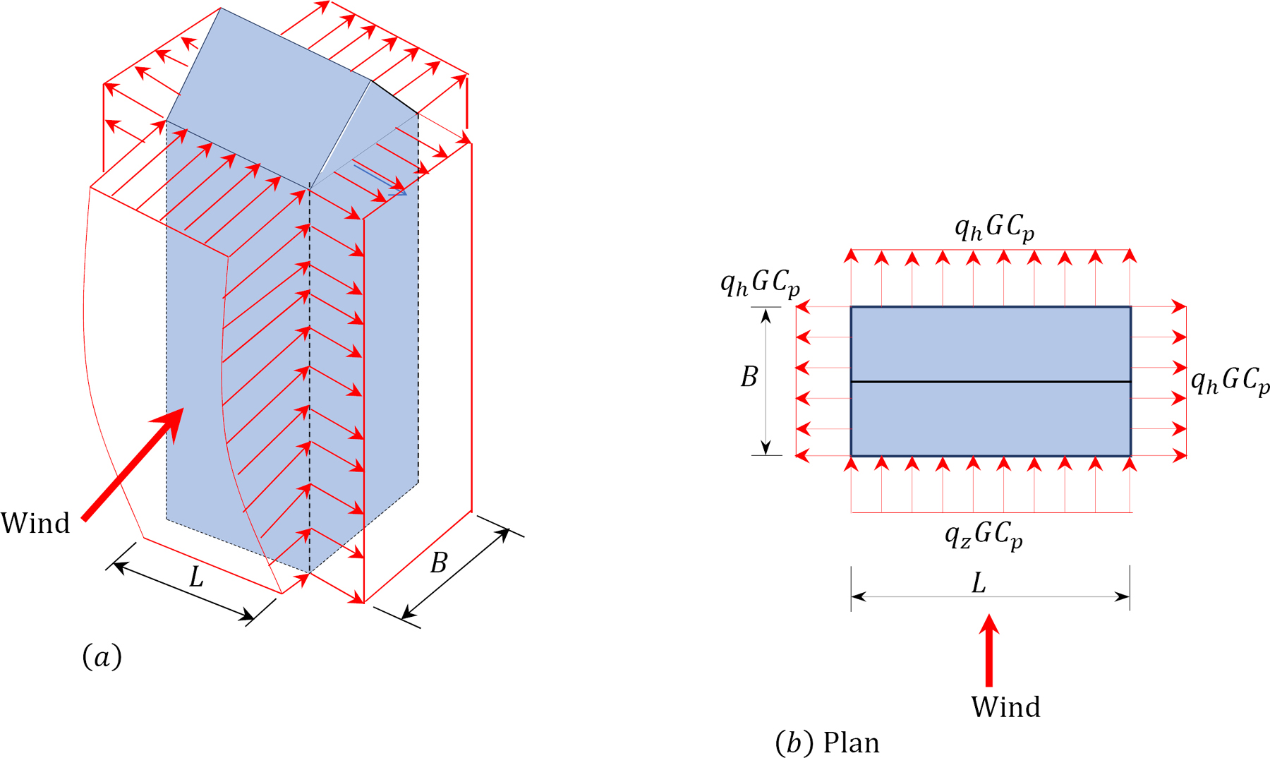
\(Fig. 2.4\). Typical wind distribution on a structureus walls and roof.

\(Table 2.6\). Wall pressure coefficient, \(C_{p \prime}\) as specified in ASCE 7-16.

Surface	L/B	Cp	Use with
Windward wall	All values	0.8	qz
Leeward wall	0-1 2 \(\geq\) 4	-0.5 -0.3 -0.2	qh
Side walls	All values	-0.7	qh

Notes:

1.Positive and negative signs are indicative of the wind pressures acting toward and away from the surfaces.

2.\(L\) is the dimension of the building normal to the wind direction, and \(B\) is the dimension parallel to the wind direction.

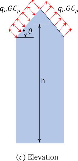
\(Table 2.7\). Roof pressure coefficients, \(C_{p \prime}\) for use with \(q_{h \prime}\) as specified in ASCE 7-16.

Wind direction	Windward angle, \(\theta\)				Leeward angle, \(\theta\)
	h/L	10°	15°	20°	10°	15°	\(\geq\)20°
Normal to ridge	\(\leq\) 0.25 0.5 \(\gt\) 1.0	-0.7 -0.9 -1.3	-0.5 -0.7 -1.0	-0.3 -0.4 -0.7	-0.3 -0.5 -0.7	-0.5 -0.5 -0.6	-0.6 -0.6 -0.6

 

Example 2.3

The two-story building shown in Figure 2.5 is an elementary school located on a flat terrain in a suburban area, with a wind speed of 102 mph and exposure category B. What is the wind velocity pressure at roof height for the main wind force resisting system (MWFRS)?

\(Fig. 2.5\). Two – story building.

Solution

The mean height of the roof is \(h=20 \mathrm{ft}\).

ASCE 7-16 states that if the exposure category is \(B\) and the velocity pressure exposure coefficient for \(h=20^{\prime}\), then \(K_{z}=0.7\).

The topography factor from section 26.8.2 of ASCE 7-16 is \(K_{z t}=1.0\).

ASCE 7-16, is \(K_{d}=0.85\).

Using equation 2.3, the velocity pressure at a roof height of \(20^{\prime}\) for the MWFRS is as follows:

\(\begin{aligned}
q_{z} &=0.00256 K_{z} K_{z t} K_{d} V^{2} \\
&=0.00256(0.7)(1.0)(0.85)(102)^{2}=15.84 \mathrm{lb} / \mathrm{ft}^{2}
\end{aligned}\)

2.1.4.3 Snow Loads

In some geographic regions, the force exerted by accumulated snow and ice on buildings’ roofs can be quite enormous, and it can lead to structural failure if not considered in structural design.

Suggested design values of snow loads are provided in codes and design specifications. The basis for the computation of snow loads is what is referred to as the ground snow load. The ground snow load is defined by the International Building Code (IBC) as the weight of snow on the ground surface. The ground snow loads for various parts of the United States can be obtained from the contour maps in ASCE 7-16. Some typical values of the ground snow loads from this standard are presented in Table 2.8. Once these loads for the required geographic areas have been established, they must be modified for specific conditions to obtain the snow load for structural design.

According to ASCE 7-16, the design snow loads for flat roofs and sloped roofs can be obtained using the following equations: \[\begin{array}{l}
p_{f}=0.7 C_{e} C_{t} I p_{g} \\
p_{s}=C_{s} p_{f}
\end{array}\]

where

\(p_{f}\) = design flat roof snow load.

\(p_{s}\) = design snow load for a sloped roof.

\(p_{g}\) = ground snow load.

\(I\) = importance factor. See Table 2.9 for importance factor values, depending on the category of the building.

\(C_{e}\) = exposure factor. See Table 2.10 for exposure factor values, depending on the terrain category.

\(C_{t}\) = thermal factor. See Table 2.11 for typical values.

\(C_{s}\) = slope factor. Values of C_s are provided in section 7.4.1 through 7.4.4 of ASCE 7-16, depending on various factors.

\(Table 2.8\). Typical ground snow loads, as specified in ASCE 7-16.

Location	Load (PSF)
Lancaster, PA Yakutat, AK New York City, NY San Francisco, CA Chicago, IL Tallahassee, FL	30 150 30 5 25 0

\(Table 2.9\). Importance factor for snow load, \(I_{S \prime}\) as specified in ASCE 7-16.

Risk Category of Structure	Importance Factor
I II III IV	0.8 1.0 1.1 1.2

\(Table 2.10\). Exposure coefficient, \(C_{e \prime}\) as specified in ASCE 7-16.

Terrain Category	Exposure of Roof
	Fully Exposed	Partially Exposed	Sheltered
A: Large city center B: Urban and suburban areas C: Open terrain with scattered obstructions D: Unobstructed areas with wind over open water Above the tree line in windswept mountainous areas Alaska in areas with trees not within two miles of the site	N/A 0.9 0.9 0.8 0.7 0.7	1.1 1.0 1.0 0.9 0.8 0.8	1.3 1.2 1.1 1.0 N/A N/A

 

\(Table 2.11\). Thermal factor, \(C_{t \prime}\) as specified in ASCE 7-16.

Thermal Condition	Thermal Factor
All structures except as indicated below	1.0
Structures kept just above freezing and others with cold, ventilated roofs in which the thermal resistance (R-value) between the ventilated space and the heated space exceeds 25° F × h × ft^2/Btu (4.4 K × m^2/W)	1.1
Unheated and open air structures	1.2
Structures intentionally kept below freezing	1.3
Continuously heated greenhouses with a roof having a thermal resistance (R-value) less than 2.0 ° F × h × ft^2/Btu	0.85

Example 2.4

A single-story heated residential building located in the suburban area of Lancaster, PA is considered partially exposed. The roof of the building slopes at 1 on 20, and it is without overhanging eaves. What is the design snow load on the roof?

Solution

ASCE 7-16, the ground snow load for Lancaster, PA is

\(p_{g}=30 \text { psf. }\).

Since \(30 \text { psf }>20 \text { psf }\), the rain-on-snow surcharge is not required.

To find the roof slope, use \(\theta=\arctan \left(\frac{1}{20}\right)=2.86^{\circ}\).

ASCE 7-16 states that the thermal factor for a heated structure is \(C_{t} = 1.0\) (see Table 2.11).

ASCE 7-16, the exposure factor for terrain category B, partially exposed is \(C_{e}=1.0\) (see Table 2.10).

ASCE 7-16 states that the importance factor \(I_{s}=1.0\) for risk category II (see Table 2.9).

According to equation 2.6, the flat roof snow load is as follows:

\(\begin{aligned}
p_{f} &=0.7 C_{e} C_{t} I p_{g} \\
&=(0.7)(1)(1)(1)(30 \mathrm{psf})=21 \mathrm{psf}
\end{aligned}\)

Since \(21 \text { psf }>20 l_{s}=(20 \text { psf })(1)=20 \text { psf }\). Therefore, the design flat roof snow load is 21 psf.

2.1.4.4 Seismic Loads

The ground motion caused by seismic forces in many geographic regions of the world can be quite significant and often damages structures. This is particularly notable in regions near active geological faults. Thus, most building codes and standards require that structures be designed for seismic forces in such areas where earthquakes are likely to occur. The ASCE 7-16 standard provides numerous analytical methods for estimating the seismic forces when designing structures. One of these methods of analysis, which will be described in this section, is referred to as the equivalent lateral force (ELF) procedure. The lateral base shear V and the lateral seismic force at any level computed by the ELF are shown in Figure 2.6. According to the procedure, the total static lateral base shear, \(V\), in a specific direction for a building is given by the following expression: \[V=\frac{S_{D 1}}{T(R / I)} W\]

where

\(V\) = lateral base shear for the building. The estimated value of V must satisfy the following condition: \[V_{\min }=0.044 S_{D S} I W<V \leq V_{\max }=\frac{s_{D S} W}{R / I}\]

\(W\) = effective seismic weight of the building. It includes total dead load of the building and its permanent equipment and partitions.

\(T\) = fundamental natural period of a building, which depends on the mass and the stiffness of the structure. It is computed using the following empirical formula: \[T=C_{t} h_{n}^{x}\]

\(C_{t}\) = building period coefficient. The value of \(C_{t} = 0.028\) for structural steel moment resisting frames, 0.016 for reinforced concrete rigid frames, and 0.02 for most other structures (see Table 2.12).

\(h_{n}\) = height of the highest level of the building, and \(x\) = 0.8 for steel rigid moment frames, 0.9 for reinforced concrete rigid frames, and 0.75 for other systems.

\(Table 2.12\). \(C_{t}\) values for various structural systems.

Structural System	Ct	x
Steel moment resisting frames Eccentrically braced frames (EBF) All other structural systems	0.028 0.03 0.02	0.8 0.75 0.75

\(S_{D I}\) = design spectral acceleration. It is estimated by using a seismic map that provides an earthquake’s intensity of design for structures at locations with \(T\) = 1 second.

\(S_{D S}\)= design spectral acceleration. It is estimated by using a seismic map that provides an earthquake’s intensity of design for structures with \(T\) = 0.2 second.

\(R\) = response modification coefficient. It accounts for the ability of a structural system to resist seismic forces. The values of \(R\) for several common systems are presented in Table 2.13.

\(I\) = importance factor. This is a measure of the consequences to human life and damage to property in the event that the structure fails. The value of the importance factor is 1 for office buildings, but equals 1.5 for hospitals, police stations, and other public buildings where loss of more life or damages to property are anticipated should a structure fail.

\(Table 2.13\). Response modification coefficient, \(R\), as specified in ASCE 7-16.

Seismic Force-Resisting System	R
Bearing wall systems Ordinary reinforced concrete shear walls Ordinary reinforced masonry shear walls Light-frame (cold-formed steel) walls sheathed with structural panels rated for shear resistance or steel sheets	4 2 6\(\frac{1}{2}\)
Building frame systems Ordinary reinforced concrete shear walls Ordinary reinforced masonry shear walls Steel buckling-restrained braced frames	5 2 8
Moment-resisting frame systems Steel special moment frames Steel ordinary moment frames Ordinary reinforced concrete moment frames	8 3\(\frac{1}{2}\) 3

Once the total seismic static lateral base shear force in a given direction for a structure has been computed, the next step is to determine the lateral seismic force that will be applied to each floor level using the following equation: \[F_{x}=\frac{W_{x} h_{x}^{k}}{\sum W_{i} h_{i}^{k}} V\]

where

\(F_{x}\) = lateral seismic force applied to level \(x\).

\(W_{i}\) and \(W_{x}\) = effective seismic weights at levels \(i\) and \(x\).

\(h_{i}\) and \(h_{x}\) = heights from the base of the structure to floors at levels \(i\) and \(x\).

\(\Sigma W_{i} h_{i}^{k}\) = summation of the product W_{i} and \(h_{i}^{k}\) over the entire structure.

\(k\) = distribution exponent related to the fundamental natural period of the structure. For \(T \leq 0.5\)s, \(k = 1.0\), and for \(T \geq 2.5\)s, \(k = 2.0\). For \(T\) lying between 0.5s and 2.5s, \(k\) can be computed using the following relationship: \[k=1+\frac{T-0.5}{2}\]

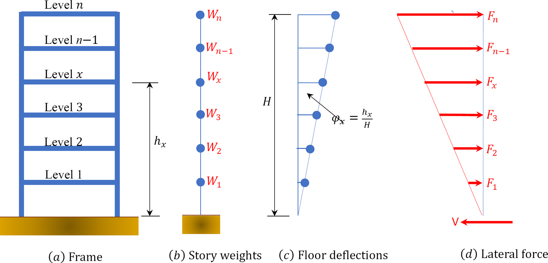
\(Fig. 2.6\). Equivalent lateral force procedure

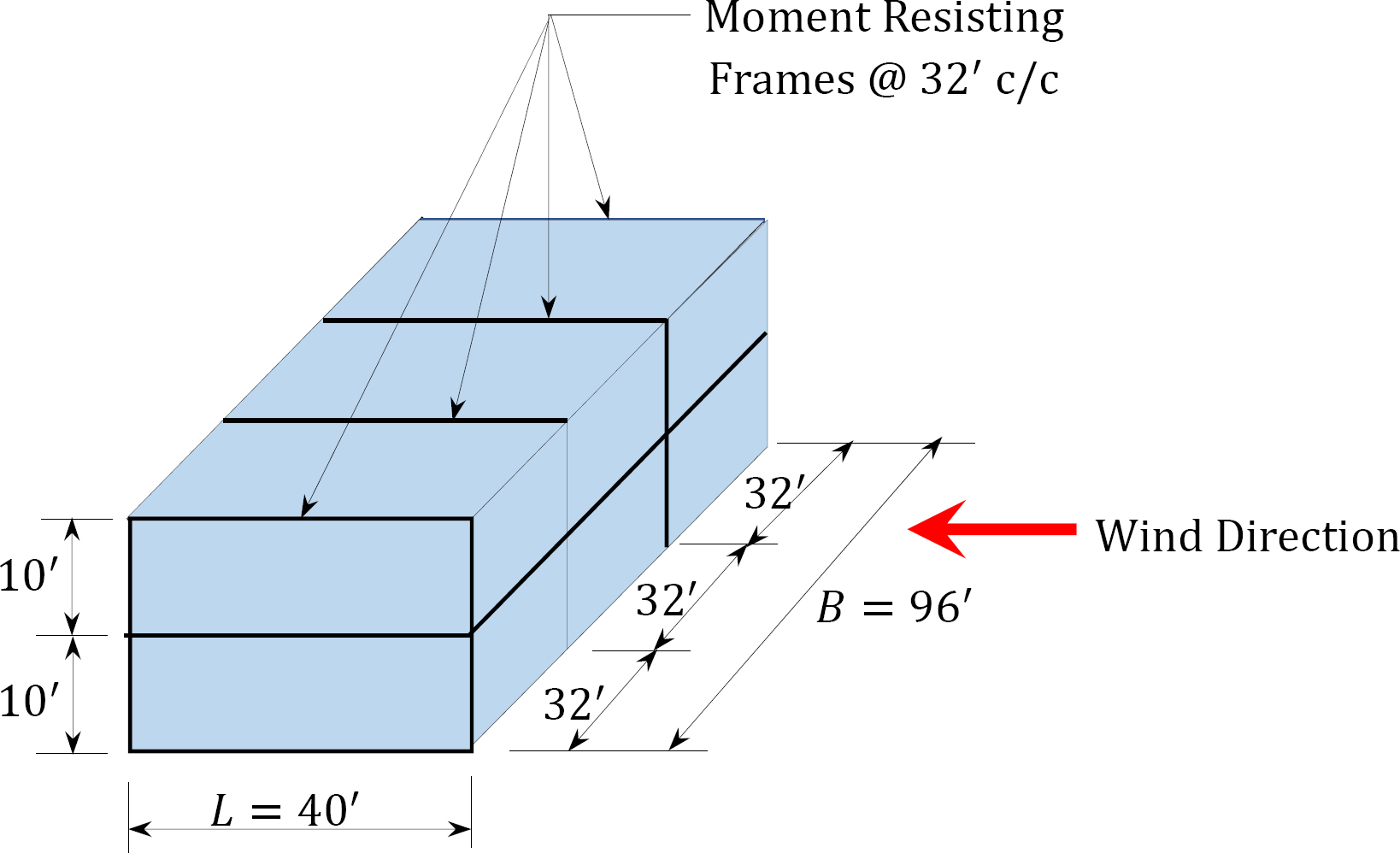
Example 2.5

The five-story office steel building shown in Figure 2.7 is laterally braced with steel special moment resisting frames, and it measures 75 ft by 100 ft in the plan. The building is located in New York City. Using the ASCE 7-16 equivalent lateral force procedure, determine the lateral force that will be applied to the fourth floor of the structure. The roof dead load is 32 psf, the floor dead load (including the partition load) is 80 psf, and the flat roof snow load is 40 psf. Ignore the weight of cladding. The design spectral acceleration parameters are \(S_{D S}) = 0.28, and \(S_{D 1}\) = 0.11.

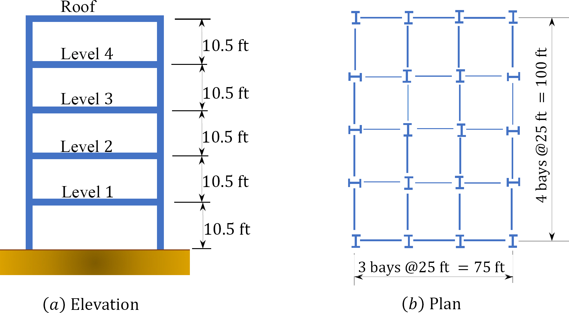
\(Fig. 2.7\). Five – story office building.

Solution

\(S_{D S}) = 0.28, and \(S_{D 1}\) = 0.11 (given).

\(R\) = 8 for special moment resisting steel frame (see Table 2.13).

An office building is in occupancy risk category II, so \(I_{e}\) = 1.0 (see Table 2.9).

Calculate the approximate fundamental natural period of the building \(T_{a}\).

\(C_{t} = 0.028\) and \(x = 0.8\) (from Table 2.12 for steel moment resisting frames).

\(h_{n}\) = Roof height = 52.5 ft

 

Determine the dead load at each level. Since the flat roof snow load given for the office building is greater than 30 psf, 20% of the snow load must be included in the seismic dead load computations.

The weight assigned to the roof level is as follows:

\(W_{\text {roof }}=(32 \mathrm{psf})(75 \mathrm{ft})(100 \mathrm{ft})+(20 \%)(40 \mathrm{psf})(75 \mathrm{ft})(100 \mathrm{ft})=300,000 \mathrm{lb}\)

The weight assigned to all other levels is as follows:

\(W_{i}=(80 \mathrm{psf})(75 \mathrm{ft})(100 \mathrm{ft})=600,000 \mathrm{lb}\)

The total dead load is as follows:

\(W_{\text {Total}}=300,000 \mathrm{lb}+(4)(600,000 \mathrm{lb})=2700 \mathrm{k}\)

Calculate the seismic response coefficient \(C_{s}\).

\(\begin{array}{l}
C_{S}=\frac{S_{D S}}{R / I_{e}}=\frac{0.28}{8 / 1.0}=0.035 \\
\leq \frac{S_{D 1}}{\left(\frac{T R}{I_{e}}\right)}=\frac{0.11}{[(0.67)(8) / 1.0]}=0.021
\end{array}\)

Therefore, \(C_{s}=0.021>0.01\)

Determine the seismic base shear \(V\).

\(V=C_{S} W=(0.021)(2700 \mathrm{kips})=56.7 \mathrm{k}\)

Calculate the lateral force applied to the fourth floor.

\(\begin{array}{l}
k=1+\frac{T-0.5}{2}=1+\frac{0.67-0.5}{2}=1.085 \\
F_{4}=\frac{W_{4} h_{4}^{k}}{\sum_{i=1}^{m} W_{i} h_{i}^{k}}(V) \\
=\frac{600(42)^{1.085}}{600(10.5)^{1.085}+600(21)^{1.085}+600(31.5)^{1.085}+600(42)^{1.085}+300(52.5)^{1.085}}(56.7 \mathrm{k}) \\
=18.51 \mathrm{k}
\end{array}\)

2.1.4.5 Hydrostatic and Earth Pressures

Retaining structures must be designed against overturning and sliding caused by hydrostatic and earth pressures to ensure the stability of their bases and walls. Examples of retaining walls include gravity walls, cantilever walls, counterfort walls, tanks, bulkheads, sheet piles, and others. The pressures developed by the retained material are always normal to the surfaces of the retaining structure in contact with them, and they vary linearly with height. The intensity of normal pressure, \(p\), and the resultant force, \(P\), on the retaining structure is computed as follows: \[\begin{aligned}
p &=\gamma h \\
P &=\frac{1}{2} \gamma h^{2}
\end{aligned}\]

Where

\(y\) = unit weight of the retained material.

\(h\) = distance from the surface of the retained material and the point under consideration.

2.1.4.6 Miscellaneous Loads

There are numerous other loads that may also be considered when designing structures, depending on specific cases. Their inclusion in the load combinations will be based on a designer’s discretion if they are perceived to have a future significant impact on structural integrity. These loads include thermal forces, centrifugal forces, forces due to differential settlements, ice loads, flooding loads, blasting loads, and more.