6.2: Cables

Cables are flexible structures that support the applied transverse loads by the tensile resistance developed in its members. Cables are used in suspension bridges, tension leg offshore platforms, transmission lines, and several other engineering applications. The distinguishing feature of a cable is its ability to take different shapes when subjected to different types of loadings. Under a uniform load, a cable takes the shape of a curve, while under a concentrated load, it takes the form of several linear segments between the load’s points of application.

General Cable Theorem

The general cable theorem states that at any point on a cable that is supported at two ends and subjected to vertical transverse loads, the product of the horizontal component of the cable tension and the vertical distance from that point to the cable chord equals the moment which would occur at that section if the load carried by the cable were acting on a simply supported beam of the same span as that of the cable.

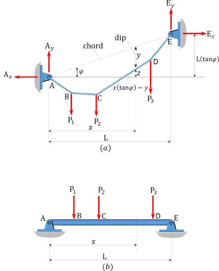
\(Fig. 6.7\). Cable (\(a\)) and beam (\(b\)).

To prove the general cable theorem, consider the cable and the beam shown in Figure 6.7a and Figure 6.7b, respectively. Both structures are supported at both ends, have a span \(L\), and are subjected to the same concentrated loads at \(B\), \(C\), and \(D\). A line joining supports \(A\) and \(E\) is referred to as the chord, while a vertical height from the chord to the surface of the cable at any point of a distance \(x\) from the left support, as shown in Figure 6.7a, is known as the dip at that point. For equilibrium of a structure, the horizontal reactions at both supports must be the same. From static equilibrium, the moment of the forces on the cable about support \(B\) and about the section at a distance \(x\) from the left support can be expressed as follows, respectively: \[\begin{array}{l}
+\curvearrowleft \sum M_{B}=0 \\
\quad \quad -A_{y} L-A_{x} L(\tan \varphi)+\sum M_{B P}=0
\end{array}\]

where

\(\Sigma M_{B P}=\) the algebraic sum of the moment of the applied forces about support \(B\).

\[\begin{array}{l}
+\curvearrowleft \sum M_{x}=0 \\
\quad \quad -A_{y} x-A_{x}[x \tan \varphi-y]+\sum M_{x P}=0
\end{array}\]

\[\text { Solving equation } 6.1 \text { suggest that } A_{y}=\frac{\left[\Sigma M_{B P}-A_{x} \text {Ltan} \varphi\right]}{L}\]

Substituting \(A_{y}\) from equation 6.8 into equation 6.7 suggests the following: \(\frac{\left[\sum M_{B P}-A_{\chi} L \tan \varphi\right] x}{L}+A_{x}(x \tan \varphi-y)=\sum M_{x P}\)

\[\begin{aligned}
&\text { or } \quad \frac{x \sum M_{B P}}{L}-x A_{x} \tan \varphi+x A_{x} \tan \varphi-A_{x} y=\sum M_{x P}\\
&\text { or } \quad A_{x} y=\frac{x \sum M_{B P}}{L}-\sum M_{x P}
\end{aligned}\]

To obtain the expression for the moment at a section \(x\) from the right support, consider the beam in Figure 6.7b. First, determine the reaction at \(A\) using the equation of static equilibrium as follows: \[\begin{aligned}
\sum M_{B} &=0 \\
A_{y} &=\frac{\sum M_{B P}}{L}
\end{aligned}\]

\[\text { The moment at a section of the beam at a distance } x \text { from support } A=A_{y} x-\sum M_{x P}\]

Substituting \(A_{y}\) from equation 6.10 into equation 6.11 suggests the following:

\[\text { The moment at section } x=\frac{x \sum M_{B P}}{L}-\sum M_{x P}\]

The moment at a section of a beam at a distance \(x\) from the left support presented in equation 6.12 is the same as equation 6.9. This confirms the general cable theorem.

Example 6.5

A cable supports two concentrated loads at \(B\) and \(C\), as shown in Figure 6.8a. Determine the sag at \(B\), the tension in the cable, and the length of the cable.

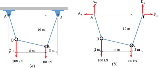
\(Fig. 6.8\). Cable.

Solution

Support reactions. The reactions of the cable are determined by applying the equations of equilibrium to the free-body diagram of the cable shown in Figure 6.8b, which is written as follows:

\(\begin{array}{l}
+\curvearrowleft \sum M_{A}=0 \\
-100(2)-80(10)+13 D_{y}=0 \\
D_{y}=76.92 \mathrm{kN} \\
+\uparrow \sum_{y}=0 \\
A_{y}+76.92-100-80=0 \\
A_{y}=103.08 \mathrm{kN} \\
+ \curvearrowleft \sum M_{C}=0 \\
-A_{x}(10)+100(8)=0 \\
A_{x}=80 \mathrm{kN} \\
+\rightarrow \sum F_{x}=0 \\
-D_{x}+80=0 \\
D_{x}=80 \mathrm{kN}
\end{array}\)

Sag at \(B\). The sag at point \(B\) of the cable is determined by taking the moment about \(B\), as shown in the free-body diagram in Figure 6.8c, which is written as follows:

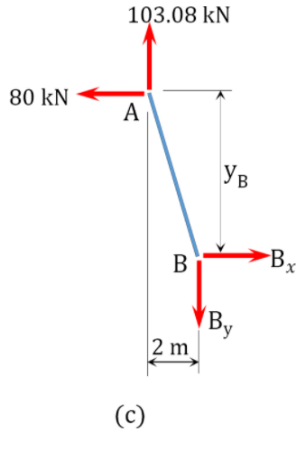
\(\begin{array}{l}
+\curvearrowleft \sum M_{B}=0 \\
-A_{y}(2)+A_{x}\left(y_{B}\right)=0 \\
y_{B}=\frac{A y(2)}{A_{x}}=\frac{103.08(2)}{80}=2.58 \mathrm{~m} \quad y_{B}=2.58 \mathrm{~m}
\end{array}\)

Tension in cable.

Tension at \(A\) and \(D\).

\(\begin{array}{l}
T_{A}=T_{A B}=\sqrt{\left(A_{y}\right)^{2}+\left(A_{x}\right)^{2}}=\sqrt{(103.08)^{2}+(80)^{2}}=130.48 \mathrm{kN} \\
T_{D}=T_{D C}=\sqrt{\left(\mathrm{D}_{y}\right)^{2}+\left(\mathrm{D}_{x}\right)^{2}}=\sqrt{(76.92)^{2}+(80)^{2}}=110.98 \mathrm{kN}
\end{array}\)

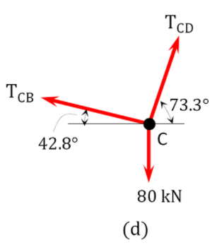
Tension in segment \(CB\).

\(\begin{array}{l}
+\rightarrow \sum F_{x}=0 \\
T_{C D} \cos 73.3^{\circ}-T_{C B} \cos 42.8^{\circ}=0 \\
T_{C B}=\frac{T_{C D} \cos \left(73.3^{\circ}\right)}{\cos 42.8}=\frac{110.98 \cos \left(73.3^{\circ}\right)}{\cos 42.8}=43.46 \mathrm{kN}
\end{array}\)

Length of cable. The length of the cable is determined as the algebraic sum of the lengths of the segments. The lengths of the segments can be obtained by the application of the Pythagoras theorem, as follows:

\(L=\sqrt{(2.58)^{2}+(2)^{2}}+\sqrt{(10-2.58)^{2}+(8)^{2}}+\sqrt{(10)^{2}+(3)^{2}}=24.62 \mathrm{~m}\)

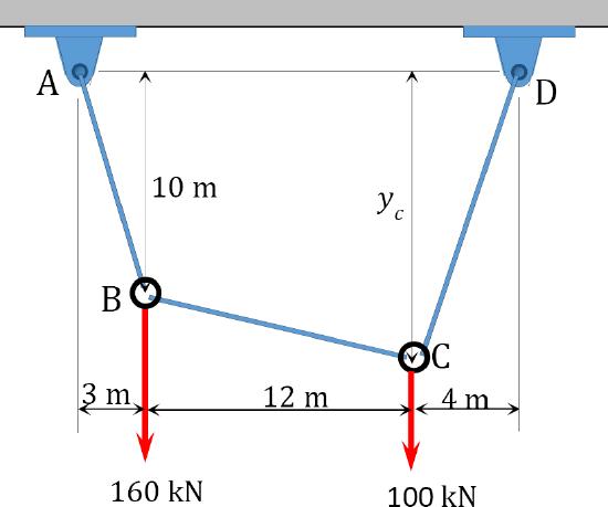
Example 6.6

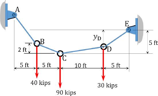
A cable supports three concentrated loads at \(B\), \(C\), and \(D\), as shown in Figure 6.9a. Determine the sag at \(B\) and \(D\), as well as the tension in each segment of the cable.

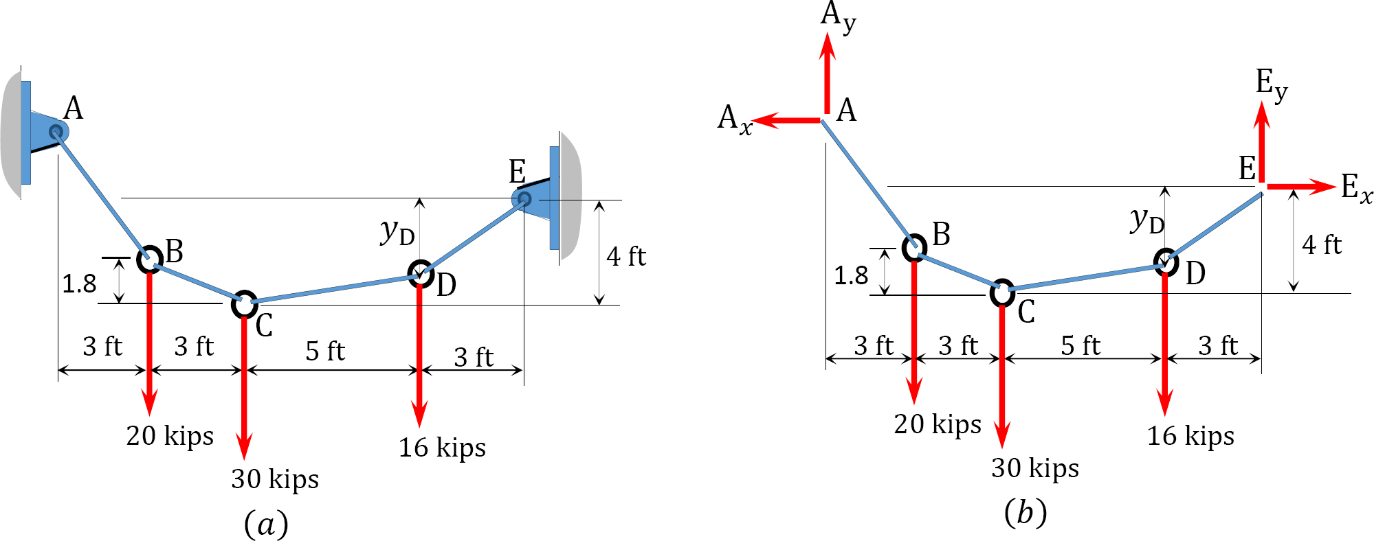
\(Fig. 6.9\). Cable.

Solution

Support reactions. The reactions shown in the free-body diagram of the cable in Figure 6.9b are determined by applying the equations of equilibrium, which are written as follows:

\(\begin{array}{l}
+\curvearrowleft \sum M_{A}=0 \\
-20(3)-30(6)-16(11)+14=0 \\
E_{y}=29.71 \text { kips } \\
+\uparrow \sum F_{y}=0 \\
A_{y}+29.71-20-30-16=0 \\
A_{y}=36.29 \text { kips } \\
+\curvearrowleft \sum M_{C}=0 \\
29.71(8)-E_{x}(4)-16(5)=0 \\
E_{x}=39.42 \text { kips } \\
+\rightarrow \sum F_{x}=0
\end{array}\)

\(-A_{X}+39.42=0\)

\(A_{x}=39.42 \text { kips }\)

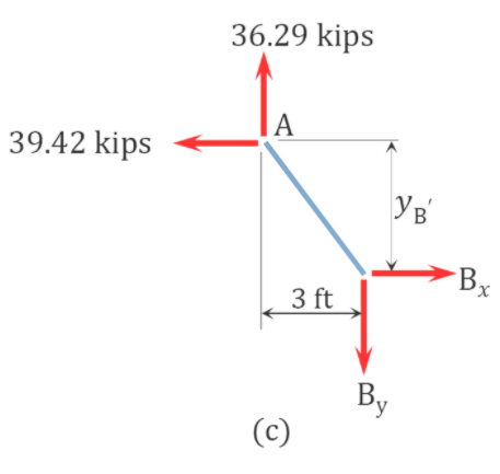
Sag. The sag at \(B\) is determined by summing the moment about \(B\), as shown in the free-body diagram in Figure 6.9c, while the sag at \(D\) was computed by summing the moment about \(D\), as shown in the free-body diagram in Figure 6.9d.

Sag at \(B\).

\(\begin{array}{l}
\curvearrowleft+\sum M_{B}=0 \\
-36.29(3)+39.42\left(y_{\mathrm{B}^{\prime}}\right)=0 \\
y_{\mathrm{B}^{\prime}}=2.76 \mathrm{ft}
\end{array}\)

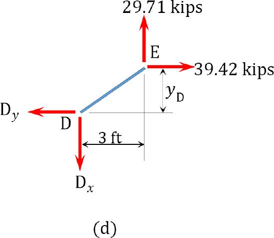
Sag at \(D\).

\(\begin{array}{l}
\curvearrowleft + \sum M_{D}=0 \\
29.71(3)+39.42\left(y_{D}\right)=0 \\
y_{D}=2.26 \mathrm{ft}
\end{array}\)

Tension.

Tension at \(A\).

\(T_{A}=T_{A B}=\sqrt{\left(A_{y}\right)^{2}+\left(A_{x}\right)^{2}}=\sqrt{(36.29)^{2}+(39.42)^{2}}=53.58 \mathrm{kips}\)

Tension at \(E\).

\(T_{E}=T_{E D}=\sqrt{\left(\mathrm{E}_{y}\right)^{2}+\left(\mathrm{E}_{x}\right)^{2}}=\sqrt{(29.71)^{2}+(39.42)^{2}}=49.36 \mathrm{kips}\)

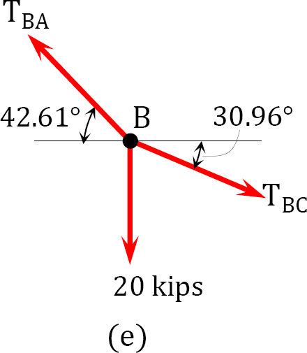
Tension at \(B\).

\(\begin{array}{l}
\rightarrow+\sum F_{x}=0 \\
-T_{B A} \cos 42.61^{\circ}+T_{B C} \cos 30.96^{\circ}=0 \\
T_{B C}=\frac{T_{B A} \cos 42.61^{\circ}}{\cos 30.96^{\circ}}=\frac{53.58 \cos 42.61^{\circ}}{\cos 30.96^{\circ}}=46 \text { kips }
\end{array}\)

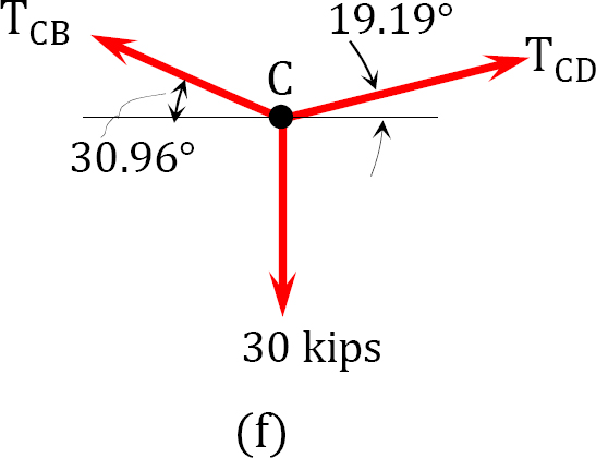
Tension at \(C\).

\(\begin{array}{l}
\rightarrow+\sum F_{x}=0 \\
-T_{C B} \cos 30.96^{\circ}+T_{C D} \cos 19.19^{\circ}=0 \\
T_{C D}=\frac{T_{C B} \cos 30.96^{\circ}}{\cos 19.19^{\circ}}=\frac{46 \cos 30.96^{\circ}}{\cos 19.19^{\circ}}=41.77 \mathrm{kips}
\end{array}\)

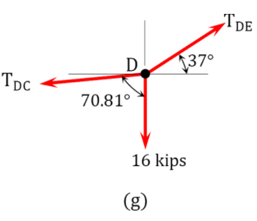
Tension at \(D\).

\(\begin{array}{l}
\rightarrow+\sum F_{x}=0 \\
-T_{D C} \sin 70.81^{\circ}+T_{D E} \cos 37^{\circ}=0 \\
T_{D E}=\frac{T_{DC} \sin \left(70.81^{\circ}\right)}{\cos 37^{\circ}}=\frac{41.77 \sin \left(70.81^{\circ}\right)}{\cos 37^{\circ}}=49.40 \mathrm{kN}
\end{array}\)

Parabolic Cable Carrying Horizontal Distributed Loads

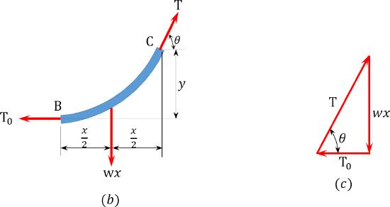
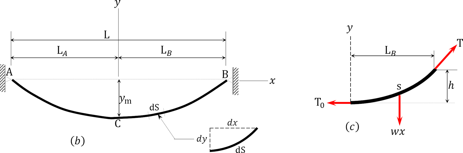
To develop the basic relationships for the analysis of parabolic cables, consider segment \(BC\) of the cable suspended from two points \(A\) and \(D\), as shown in Figure 6.10a. Point \(B\) is the lowest point of the cable, while point \(C\) is an arbitrary point lying on the cable. Taking \(B\) as the origin and denoting the tensile horizontal force at this origin as \(T_{0}\) and denoting the tensile inclined force at \(C\) as \(T\), as shown in Figure 6.10b, suggests the following:

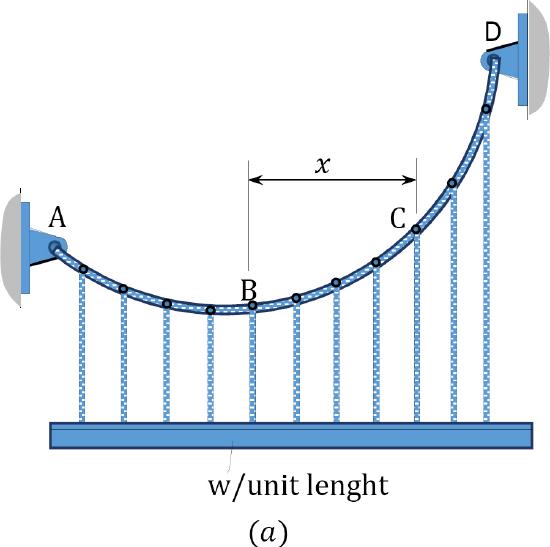
\(Fig. 6.10\). Suspended cable.

Figure 6.10c suggests the following: \[\tan \theta=\frac{d y}{d x}=\frac{w x}{T_{0}}\]

Equation 6.13 defines the slope of the curve of the cable with respect to \(x\). To determine the vertical distance between the lowest point of the cable (point \(B\)) and the arbitrary point \(C\), rearrange and further integrate equation 6.13, as follows: \[\begin{array}{l}
\quad d y=\frac{w x}{T_{0}} d x \\
\int_{0}^{y} d y=\int_{0}^{x} \frac{w x}{T_{0}} d x \\
y=\frac{w x^{2}}{2 T_{0}}
\end{array}\]

Summing the moments about \(C\) in Figure 6.10b suggests the following:

\(\begin{array}{l}
\curvearrowleft+\sum M_{c} \\
w x\left(\frac{x}{2}\right)-T_{0} y=0 \\
\text { Therefore, } y=\frac{w x^{2}}{2 T_{0}}
\end{array}\)

Applying Pythagorean theory to Figure 6.10c suggests the following: \[T=\sqrt{\left(T_{0}\right)^{2}+(w x)^{2}}\]

where

\(T\) and \(T_{0}\) are the maximum and minimum tensions in the cable, respectively.

Example 6.7

A cable supports a uniformly distributed load, as shown Figure 6.11a. Determine the horizontal reaction at the supports of the cable, the expression of the shape of the cable, and the length of the cable.

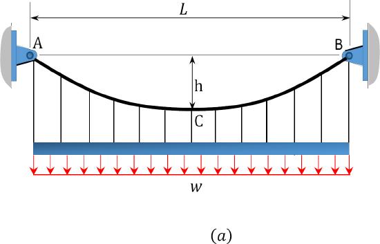
\(Fig. 6.11\). Cable with uniformly distributed load.

Solution

As the dip of the cable is known, apply the general cable theorem to find the horizontal reaction.

\(\text { At point } C, x=\frac{\mathrm{L}}{2}, y=h\)

The expression of the shape of the cable is found using the following equations:

\(\begin{array}{l}
\sum M_{x P}=\left(\frac{w L}{2}\right)\left(\frac{L}{4}\right)=\frac{w \mathrm{~L}^{2}}{8} \\
\sum M_{B P}=\frac{w \mathrm{~L}^{2}}{2} \\
A_{x} h=\left(\frac{1 / 2 L}{L}\right)\left(\frac{w L^{2}}{2}\right)-\left(\frac{w L^{2}}{8}\right) \\
A_{x}=\frac{w L^{2}}{8 h}
\end{array}\)

For any point \(\mathrm{P}(x, y)\) on the cable, apply cable equation.

The moment at any section \(x\) due to the applied load is expressed as follows:

\(\sum M_{x}=\frac{w x^{2}}{2}\)

The moment at support \(B\) is written as follows:

\(\sum M_{B}=\frac{w L^{2}}{2}\)

Applying the general cable theorem yields the following:

\(\begin{aligned}
A_{x} y &=\left(\frac{x}{L}\right)\left(\frac{w L^{2}}{2}\right)-\frac{w x^{2}}{2} \\
&=\left(\frac{w}{2}\right)(x)(L-x) \\
\left(\frac{w L^{2}}{8 h}\right) y=&\left(\frac{w}{2}\right)(x)(L-x) \\
y &=\frac{4 h}{L^{2}} x(L-x)
\end{aligned}\)

The length of the cable can be found using the following:

\(\begin{array}{l}
(d S)^{2}=(d x)^{2}+(d y)^{2} \\
(d S)^{2}=(d x)^{2}\left[1+\left(\frac{d y}{d x}\right)^{2}\right]
\end{array}\)

\[\begin{array}{l}
S=\sqrt{1+\left(\frac{d y}{d x}\right)^{2}} d x \\
S=\int_{0}^{L_{B}} d S=\int_{0}^{L_{B}} \sqrt{1+\left(\frac{d y}{d x}\right)^{2}} d x=\int_{0}^{L_{B}} \sqrt{1+\left(\frac{w x}{T_{0}}\right)^{2}} d x
\end{array}\]

The solution of equation 6.16 can be simplified by expressing the radical under the integral as a series using a binomial expansion, as presented in equation 6.17, and then integrating each term. \[\sqrt{1+a}=(1+a)^{1 / 2}=1+\frac{1}{2} a-\frac{1}{8} a^{2}+\frac{1}{16} a^{3}-+\frac{5}{128} a^{4}+\frac{7}{256} a^{5}-\cdots\]

Putting \(a=\left(\frac{w x}{T_{0}}\right)^{2}\) into three terms of the expansion in equation 6.13 suggests the following: \[\sqrt{1+\left(\frac{w x}{T_{0}}\right)^{2}}=1+\frac{1}{2}\left(\frac{w}{T_{0}}\right)^{2} \mathrm{X}^{2}-\frac{1}{8}\left(\frac{w}{T_{0}}\right)^{4} X^{4}\]

Thus, equation 6.16 can be written as the following: \[\begin{array}{l}
S=\int_{0}^{L_{B}} d S=\int_{0}^{L_{B}} \sqrt{1+\left(\frac{d y}{d x}\right)^{2}} d x=\int_{0}^{L_{B}}\left[1+\frac{1}{2}\left(\frac{w}{T_{0}}\right)^{2} X^{2}-\frac{1}{8}\left(\frac{w}{T_{0}}\right)^{4} X^{4}\right] d x \\
=\left.\left[X+\frac{1}{6}\left(\frac{w}{T_{0}}\right)^{2} X^{3}-\frac{1}{40}\left(\frac{w}{T_{0}}\right)^{4} X^{5}\right]\right|_{0} ^{L_{B}} \\
=L_{B}+\frac{1}{6}\left(\frac{w}{T_{0}}\right)^{2} L_{B}^{3}-\frac{1}{40}\left(\frac{w}{T_{0}}\right)^{4} L_{B}^{5}
\end{array}\]

Putting \(T_{0}=\frac{w L_{B}^{2}}{2 h}\) into equation 6.19 suggests: \[\begin{aligned}
S &=L_{B}+\frac{4 h^{2}}{6 L_{B}}-\frac{16 h^{4}}{40 L_{B}^{3}} \\
&=L_{B}\left[1+\frac{2}{3}\left(\frac{h}{L_{B}}\right)^{2}-\frac{2}{5}\left(\frac{h}{L_{B}}\right)^{4}\right]
\end{aligned}\]

Example 6.8

A cable subjected to a uniform load of 240 N/m is suspended between two supports at the same level 20 m apart, as shown in Figure 6.12. If the cable has a central sag of 4 m, determine the horizontal reactions at the supports, the minimum and maximum tension in the cable, and the total length of the cable.

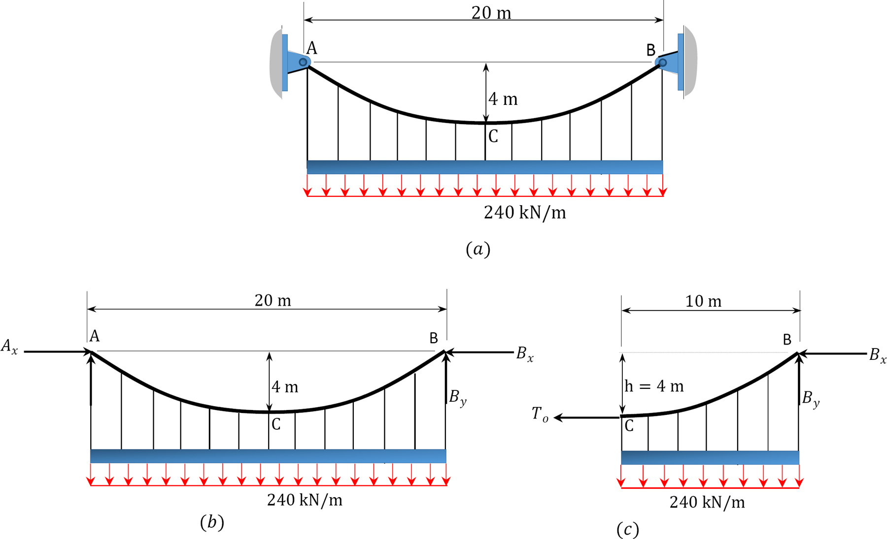
\(Fig. 6.12\). Cable.

Solution

Horizontal reactions. Applying the general cable theorem at point \(C\) suggests the following:

when \(x=\frac{L}{2}\), \(h=4 \mathrm{~m}\)

\(\begin{array}{l}
+\curvearrowleft \sum M_{x}=\frac{w L^{2}}{8}=\frac{240(20)^{2}}{8}=12000 \mathrm{Nm} \\
+\curvearrowleft \sum M_{B}=\frac{w L^{2}}{2}=\frac{240(20)^{2}}{2}=48000 \mathrm{Nm}
\end{array}\)

\(\begin{array}{r}
A_{x}(4)=48000-12000 \\
A_{x}=B_{x}=9000 \mathrm{~N}
\end{array}\)

Minimum and maximum tension. From the free-body diagram in Figure 6.12c, the minimum tension is as follows:

\(\begin{array}{l}
\curvearrowleft + \sum M_{c} \\
w x\left(\frac{x}{2}\right)-T_{0} h=0
\end{array}\)

Therefore, \(T_{0}=\frac{w x^{2}}{2 h}=\frac{240(10)^{2}}{2(4)}=3000 \mathrm{~N}\)

From equation 6.15, the maximum tension is found, as follows:

\(T_{\max }=\sqrt{\left(T_{0}\right)^{2}+(w x)^{2}}=\sqrt{(3000)^{2}+(240 \times 10)^{2}}=3841.87 \mathrm{~N}\)

The total length of cable:

\(\begin{aligned}
S &=(2)(10)\left[1+\frac{2}{3}\left(\frac{4}{10}\right)^{2}-\frac{2}{5}\left(\frac{4}{10}\right)^{4}\right] \\
&=(20)\left[1+\frac{2}{3}\left(\frac{4}{10}\right)^{2}-\frac{2}{5}\left(\frac{4}{10}\right)^{4}\right] \\
&=21.93 \mathrm{~m}
\end{aligned}\)

Chapter Summary

Internal forces in arches and cables: Arches are aesthetically pleasant structures consisting of curvilinear members. They are used for large-span structures. The presence of horizontal thrusts at the supports of arches results in the reduction of internal forces in it members. The lesser shear forces and bending moments at any section of the arches results in smaller member sizes and a more economical design compared with beam design.

Arches: Arches can be classified as two-pinned arches, three-pinned arches, or fixed arches based on their support and connection of members, as well as parabolic, segmental, or circular based on their shapes. Arches can also be classified as determinate or indeterminate. Three-pinned arches are determinate, while two-pinned arches and fixed arches, as shown in Figure 6.1, are indeterminate structures.

Cables: Cables are flexible structures in pure tension. They are used in different engineering applications, such as bridges and offshore platforms. They take different shapes, depending on the type of loading. Under concentrated loads, they take the form of segments between the loads, while under uniform loads, they take the shape of a curve, as shown below.

Some numerical examples have been solved in this chapter to demonstrate the procedures and theorem for the analysis of arches and cables.

Practice Problems

6.1 Determine the reactions at supports \(B\) and \(E\) of the three-hinged circular arch shown in Figure P6.1.

\(Fig. P6.1\). Three – hinged circular arch.

6.2 Determine the reactions at supports \(A\) and \(B\) of the parabolic arch shown in Figure P6.2. Also draw the bending moment diagram for the arch.

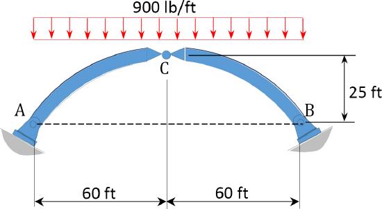
\(Fig. P6.2\). Parabolic arch.

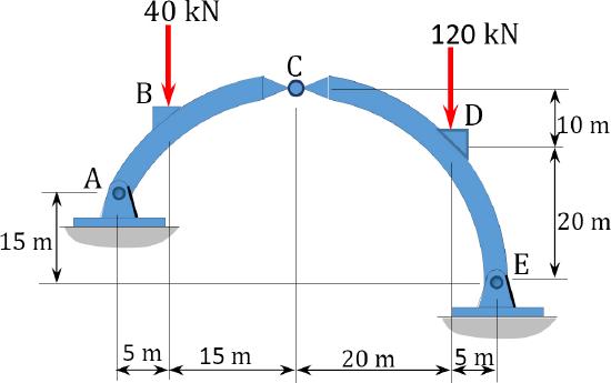
6.3 Determine the shear force, axial force, and bending moment at a point under the 80 kN load on the parabolic arch shown in Figure P6.3.

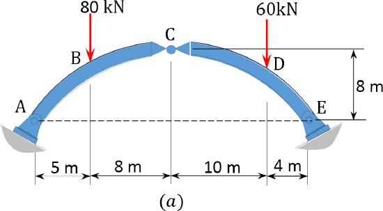
\(Fig. P6.3\). Parabolic arch.

6.4 In Figure P6.4, a cable supports loads at point \(B\) and \(C\). Determine the sag at point \(C\) and the maximum tension in the cable.

\(Fig. P6.4\). Cable.

6.5 A cable supports three concentrated loads at points \(B\), \(C\), and \(D\) in Figure P6.5. Determine the total length of the cable and the length of each segment.

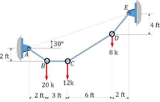
\(Fig. P6.5\). Cable.

6.6 A cable is subjected to the loading shown in Figure P6.6. Determine the total length of the cable and the tension at each support.

\(Fig. P6.6\). Cable.

6.7 A cable shown in Figure P6.7 supports a uniformly distributed load of 100 kN/m. Determine the tensions at supports \(A\) and \(C\) at the lowest point \(B\).

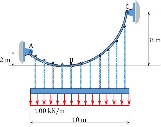
\(Fig. P6.7\). Cable.

6.8 A cable supports a uniformly distributed load in Figure P6.8. Find the horizontal reaction at the supports of the cable, the equation of the shape of the cable, the minimum and maximum tension in the cable, and the length of the cable.

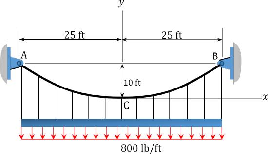
\(Fig. P6.8\). Cable.

6.9 A cable subjected to a uniform load of 300 N/m is suspended between two supports at the same level 20 m apart, as shown in Figure P6.9. If the cable has a central sag of 3 m, determine the horizontal reactions at the supports, the minimum and maximum tension in the cable, and the total length of the cable.

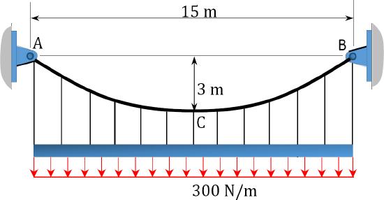
\(Fig. P6.9\). Cable.