7.2: Derivation of the Equation of the Elastic Curve of a Beam

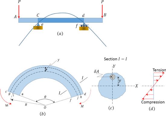
The elastic curve of a beam is the axis of a deflected beam, as indicated in Figure 7.1a.

\(Fig. 7.1\). The elastic curve of a beam.

To derive the equation of the elastic curve of a beam, first derive the equation of bending.

Consider the portion \(cdef\) of the beam shown in Figure 7.1a, subjected to pure moment, \(M\), for the derivation of the equation of bending. Due to the applied moment \(M\), the fibers above the neutral axis of the beam will elongate, while those below the neutral axis will shorten. Let \(O\) be the center and \(R\) be the radius of the beam’s curvature, and let \(ij\) be the axis of the curved beam. The beam subtends an angle \(\theta\) at \(O\). And let \(\sigma\) be the longitudinal stress in a filament \(gh\) at a distance \(y\) from the neutral axis.

From geometry, the length of the neutral axis of the beam \(ij\) and that of the filament \(gh\), located at a distance \(y\) from the neutral axis of the beam, can be computed as follows:

\(i j=R \theta \text { and } g h=(R+y) \theta\)

The strain \(\varepsilon\) in the filament can be computed as follows: \[\varepsilon=\frac{g h-i j}{i j}=\frac{(R+y) \theta-R \theta}{R \theta}=\frac{y \theta}{R \theta}=\frac{y}{R}\]

For a linear elastic material, in which Hooke’s law applies, equation 7.1 can be written as follows: \[\frac{\sigma}{E}=\frac{y}{R}\]

If an elementary area \(\delta A\) at a distance \(y\) from the neutral axis of the beam (see Figure 7.1c) is subjected to a bending stress \(\sigma\), the elemental force on this area can be computed as follows: \[\delta P=\sigma \delta A\]

The force on the entire cross-section of the beam then becomes: \[P=\int \sigma \delta A\]

From static equilibrium consideration, the external moment \(M\) in the beam is balanced by the moments about the neutral axis of the internal forces developed at a section of the beam. Thus, \[M=\int(\sigma \delta A) y\]

Substituting \(\sigma=\frac{E y}{R}\) from equation 7.2 into equation 7.5 suggests the following: \[\begin{aligned}
M &=\int\left(\frac{E}{R}\right)(y)(y)(\delta A) \\
&=\left(\frac{E}{R}\right) \int y^{2} \delta A
\end{aligned}\]

Putting \(I=\int y^{2} \delta A\) into equation 7.6 suggests the following: \[M=\frac{E I}{R}\]

where

\(I = \) the moment of inertia or the second moment of area of the section.

Combining equations 7.2 and 7.7 suggests the following: \[\frac{M}{I}=\frac{E}{R}\]

The equation of the elastic curve of a beam can be found using the following methods.

From differential calculus, the curvature at any point along a curve can be expressed as follows: \[\frac{1}{R}=\frac{\frac{d^{2} y}{d x^{2}}}{\left[1+\left(\frac{d y}{d x}\right)^{2}\right]^{3 / 2}}\]

where

\(\frac{d y}{d x} \text { and } \frac{d^{2} y}{d x^{2}}\) are the first and second derivative of the function representing the curve in terms of the Cartesian coordinates \(x\) and \(y\).

Since the beam in Figure 7.1 is assumed to be homogeneous and behaves in a linear elastic manner, its deflection under bending is small. Therefore, the quantity \(\frac{d y}{d x}\), which represents the slope of the curve at any point of the deformed beam, will also be small. Since \(\left(\frac{d y}{d x}\right)^{2}\) is negligibly insignificant, equation 7.9 could be simplified as follows: \[\frac{1}{R}=\frac{\frac{d^{2} y}{d x^{2}}}{[1+0]^{3 / 2}}=\frac{d^{2} y}{d x^{2}}\]

Combining equations 7.2 and 7.10 suggests the following: \[\frac{1}{R}=\frac{M}{E I}=\frac{d^{2} y}{d x^{2}}\]

Rearranging equation 7.11 yields the following: \[E I \frac{d^{2} y}{d x^{2}}=M\]

Equation 7.12 is referred to as the differential equation of the elastic curve of a beam.