7.6: Deflection by the Conjugate Beam Method

The conjugate beam method, developed by Heinrich Muller-Breslau in 1865, is one of the methods used to determine the slope and deflection of a beam. The method is based on the principle of statics.

A conjugate beam is defined as a fictitious beam whose length is the same as that of the actual beam, but with a loading equal to the bending moment of the actual beam divided by its flexural rigidity, \(EI\).

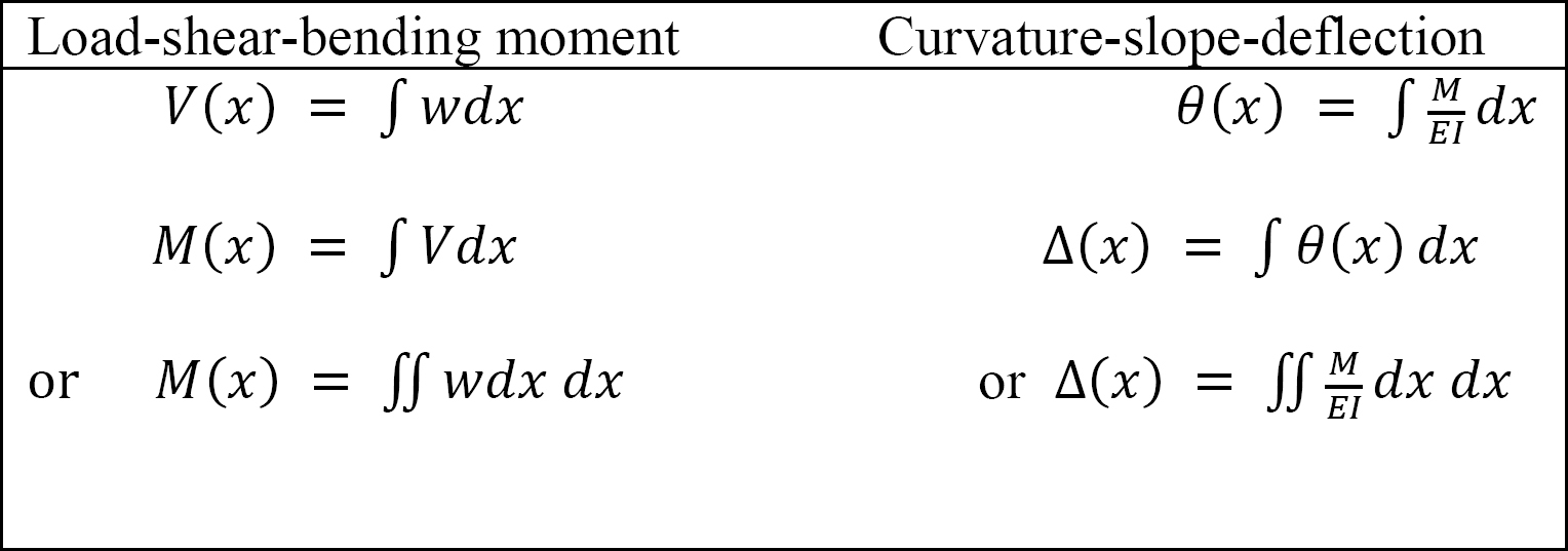
The conjugate beam method takes advantage of the similarity of the relationship among load, shear force, and bending moment, as well as among curvature, slope, and deflection derived in previous chapters and presented in Table 7.2.

\(Table 7.2\). Relationship between load-shear-bending moment and curvature-slope-deflection.

Supports for Conjugate Beams

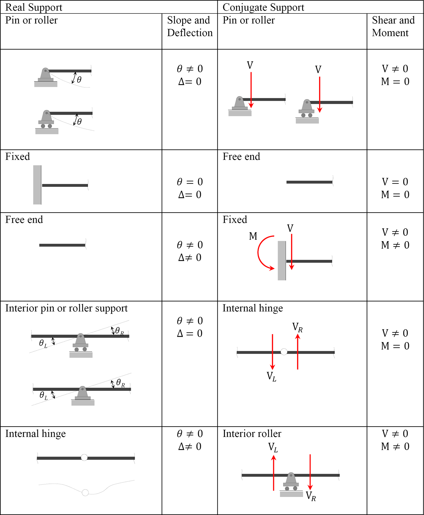
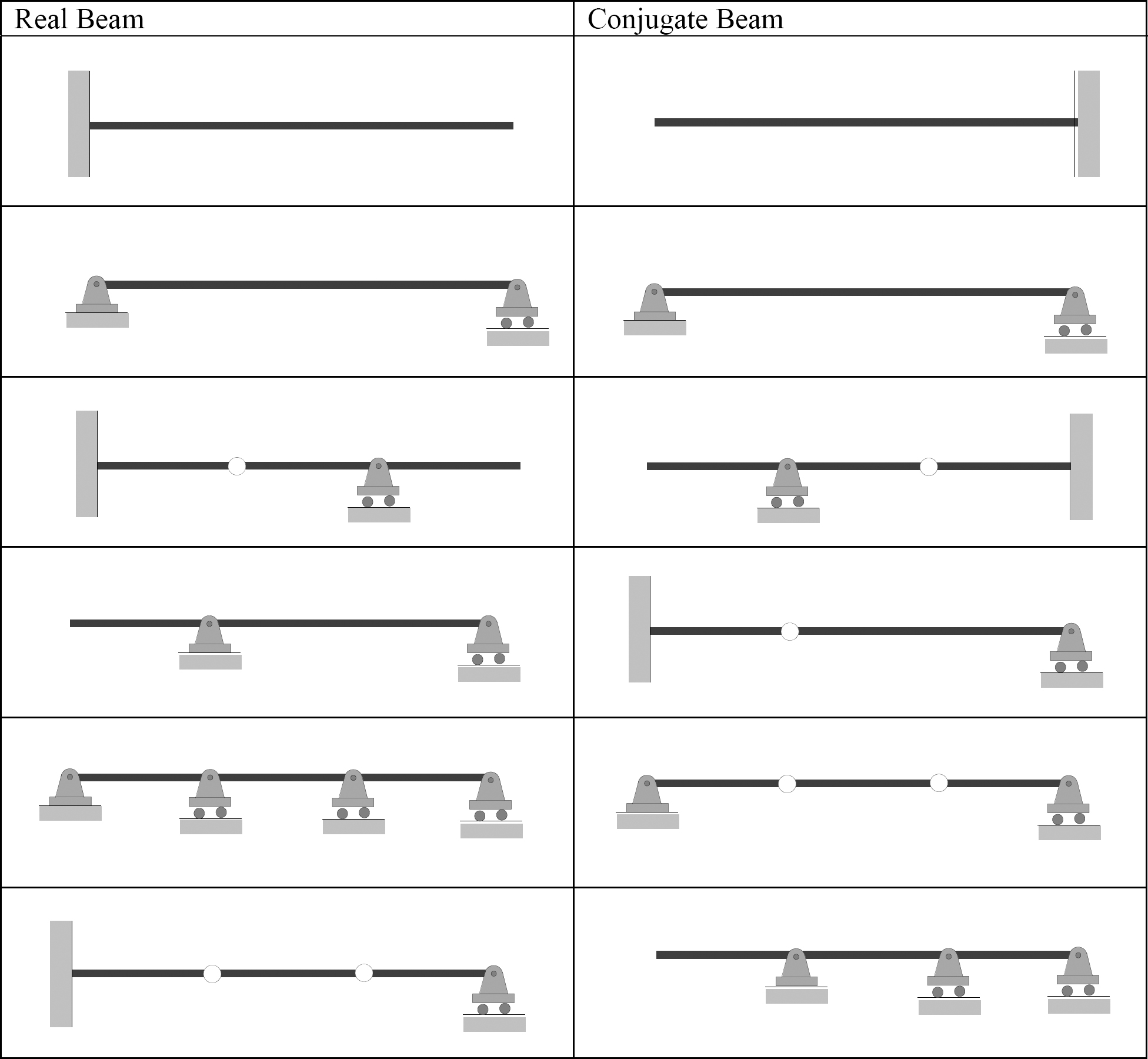
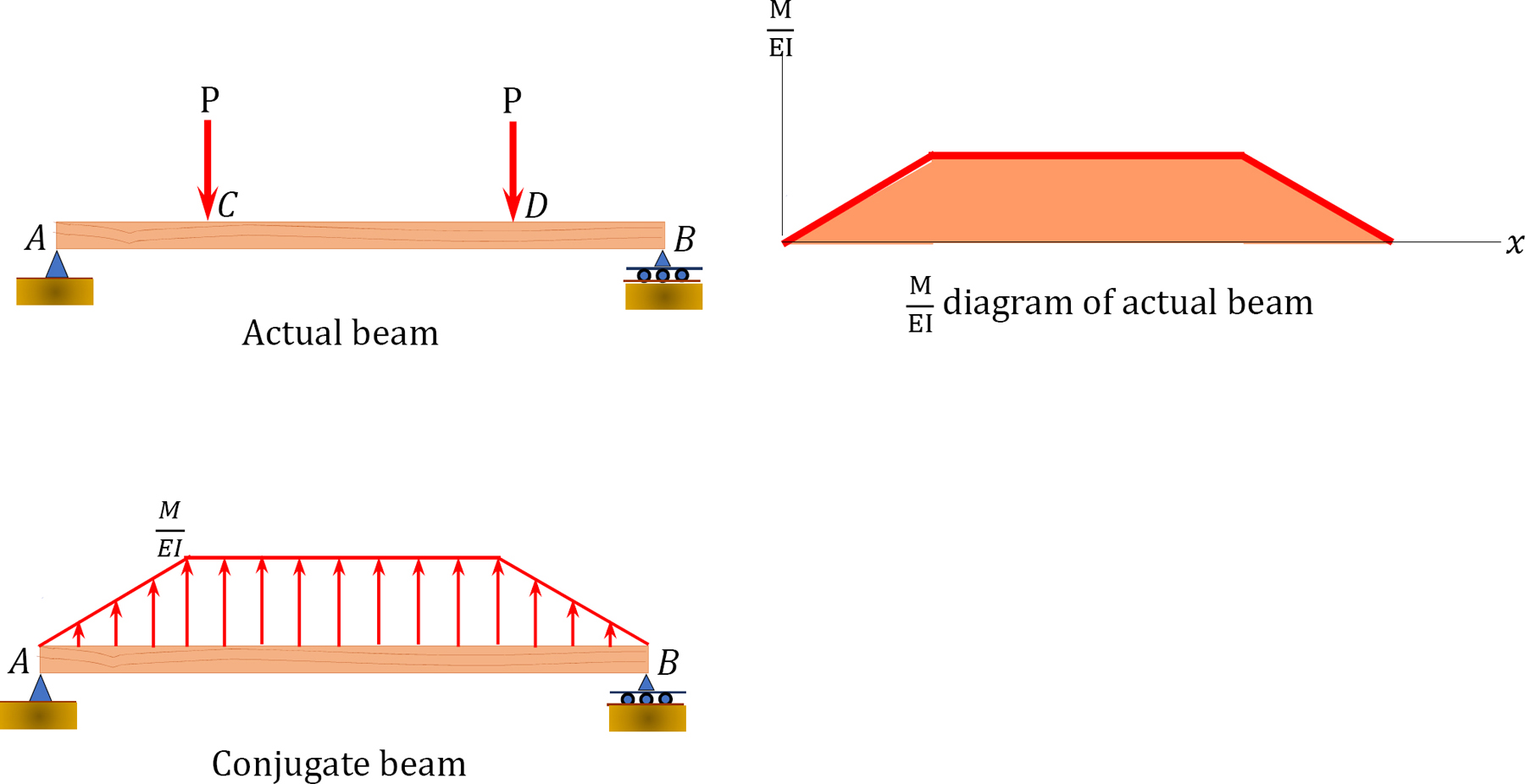
The supports for conjugate beams are shown in Table 7.3 and the examples of real and conjugate beams are shown in Figure 7.4.

\(Table 7.3\). Supports for conjugate beams.

\(Table 7.4\) Real beams and their conjugate.

Sign Convention

For a positive curvature diagram, where there is a positive ordinate of the \(\frac{M}{E I}\) diagram, the load in the conjugate should point in the positive \(y\) direction (upward) and vice versa (see Figure 7.14).

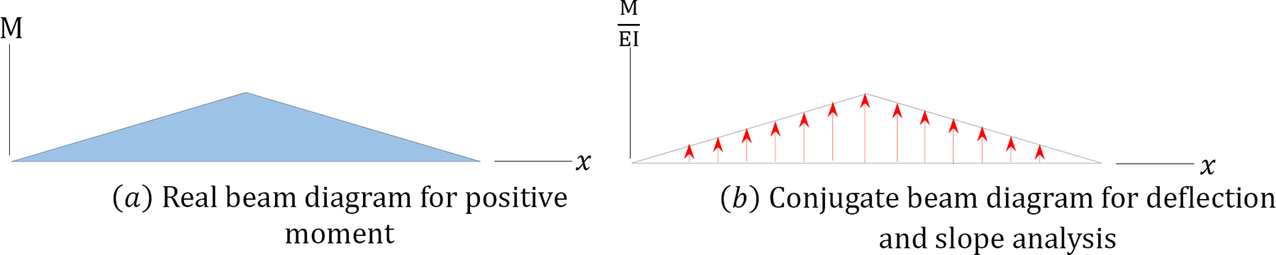
\(Fig. 7.14\). Positive curvature diagram.

If the convention stated for positive curvature diagrams is followed, then a positive shear force in the conjugate beam equals the positive slope in the real beam, and a positive moment in the conjugate beam equals a positive deflection (upward movement) of the real beam. This is shown in Figure 7.15.

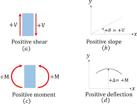
\(Fig. 7.15\). Shear and slope in beam.

Procedure for Analysis by Conjugate Beam Method

•Draw the curvature diagram for the real beam.

•Draw the conjugate beam for the real beam. The conjugate beam has the same length as the real beam. A rotation at any point in the real beam corresponds to a shear force at the same point in the conjugate beam, and a displacement at any point in the real beam corresponds to a moment in the conjugate beam.

•Apply the curvature diagram of the real beam as a distributed load on the conjugate beam.

•Using the equations of static equilibrium, determine the reactions at the supports of the conjugate beam.

•Determine the shear force and moment at the sections of interest in the conjugate beam. These shear forces and moments are equal to the slope and deflection, respectively, in the real beam. Positive shear in the conjugate beam implies a counterclockwise slope in the real beam, while a positive moment denotes an upward deflection in the real beam.

Example 7.11

Using the conjugate beam method, determine the slope and the deflection at point \(A\) of the cantilever beam shown in the Figure 7.16a. \(E = 29,000 \mathrm{ksi}\) and \(I = 280 \mathrm{in.}^{4}\)

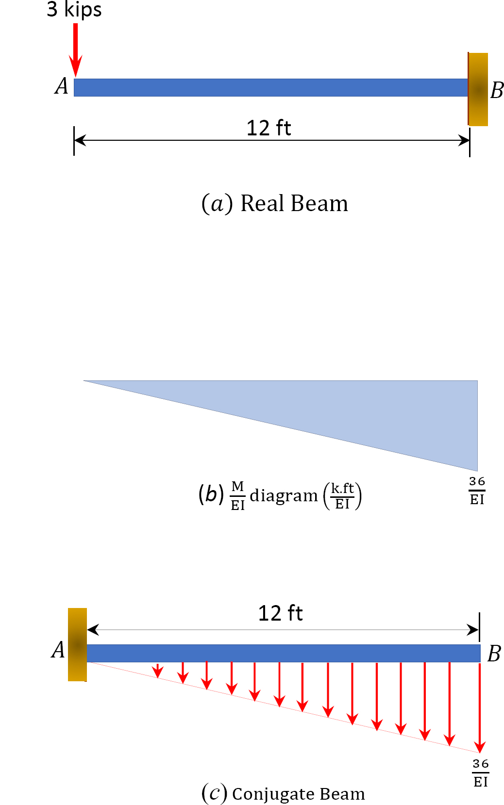
\(Fig. 7.16\). Conjugate beam.

Solution

(\(M/EI\)) diagram. First, draw the bending moment diagram for the beam and divide it by the flexural rigidity, \(EI\), to obtain the \(\frac{M}{E I}\) diagram shown in Figure 7.16b.

Conjugate beam. The conjugate beam loaded with the \(\frac{M}{E I}\) diagram is shown in Figure 7.16c. Notice that the free end in the real beam becomes fixed in the conjugate beam, while the fixed end in the real beam becomes free in the conjugate beam. The \(\frac{M}{E I}\) diagram is applied as a downward load in the conjugate beam because it is negative in Figure 7.16b.

Slope at \(A\). The slope at \(A\) in the real beam is the shear at \(A\) in the conjugate beam. The shear at \(A\) in the conjugate is as follows:

\(V_{A}=\left(\frac{1}{2}\right)(12)\left(\frac{36}{E I}\right)=\frac{216 \mathrm{k}-\mathrm{ft}^{2}}{E I}\)

The same sign convention for shear force used in Chapter 4 is used here.

Thus, the slope in the real beam at point \(A\) is as follows:

\(\theta_{\mathrm{A}}=\frac{216 \mathrm{k}-\mathrm{ft}^{2}}{E I}=\frac{216(12)^{2}}{(29,000)(280)}=0.0038 \mathrm{rad}\)

Deflection at \(A\). The deflection at \(A\) in the real beam equals the moment at \(A\) of the conjugate beam. The moment at \(A\) of the conjugate beam is as follows:

\(M_{A}=-\left(\frac{1}{2}\right)(12)\left(\frac{36}{E I}\right)\left(\frac{2}{3} \times 12\right)=-\frac{1728 \mathrm{k}-\mathrm{ft}^{3}}{E I}\)

The same sign convention for bending moment used in Chapter 4 is used here.

Thus, the deflection in the real beam at point \(A\) is as follows:

\(\Delta_{\mathrm{A}}=-\frac{1728(12)^{3}}{(29,000)(280)}=-0.37 \mathrm{in} \quad \Delta_{A}-0.37 \mathrm{in} \downarrow\)

Example 7.12

Using the conjugate beam method, determine the slope at support \(A\) and the deflection under the concentrated load of the simply supported beam at \(B\) shown in Figure 7.17a.

\(E = 29,000 \mathrm{ksi}\) and \(I = 800 \mathrm{in.}^{4}\)

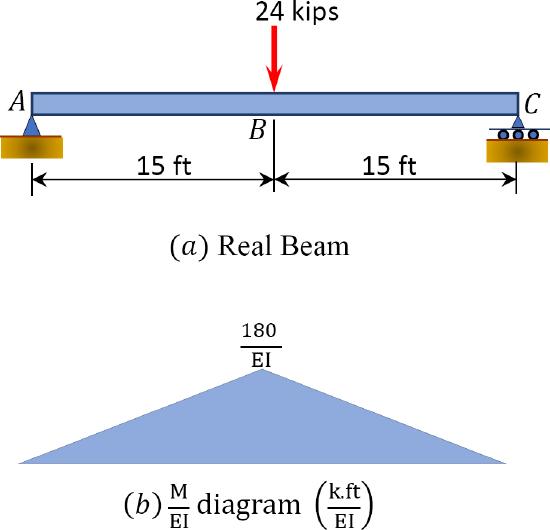
\(Fig. 7.17\). Simply supported beam.

Solution

(\(M/EI\)) diagram. First, draw the bending moment diagram for the beam and divide it by the flexural rigidity, \(EI\), to obtain the moment curvature (\(\frac{M}{E I}\)) diagram shown in Figure 7.17b.

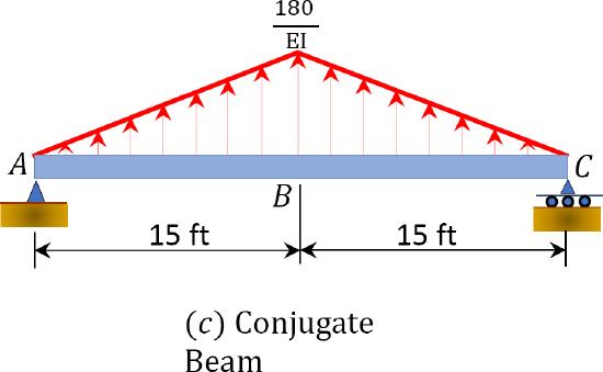
Conjugate beam. The conjugate beam loaded with the \(\frac{M}{E I}\) diagram is shown in Figure 7.17c. Notice that \(A\) and \(C\), which are simple supports in the real beam, remain the same in the conjugate beam. The \(\frac{M}{E I}\) diagram is applied as an upward load in the conjugate beam because it is positive in Figure 7.17b.

Reactions for conjugate beam. The reaction at supports of the conjugate beam can be determined as follows:

\(A_{y}=B_{y}=-\frac{1}{E I}\left(\frac{1}{2}\right)(30)(180)(0.5)=-\frac{1350 \mathrm{k} . \mathrm{ft}^{2}}{E I} \text { due to symmetry in loading }\)

Slope at \(A\). The slope at \(A\) in the real beam is the shear force at \(A\) in the conjugate beam. The shear at \(A\) in the conjugate beam is as follows:

\(V_{A}=-\frac{1350 \mathrm{k} \cdot \mathrm{ft}^{2}}{E I}\)

Thus, the slope at support \(A\) of the real beam is as follows:

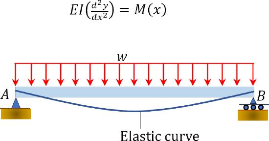
\(\theta_{A}=-\frac{1350 \mathrm{k} \cdot \mathrm{ft}^{2}}{E I}=-\frac{1350(12)^{2}}{(29,000)(800)}=-0.0084 \mathrm{rad}\)

Deflection at \(B\). The deflection at \(B\) in the real beam equals the moment at \(B\) of the conjugate beam. The moment at \(B\) of the conjugate beam is as follows:

\(M_{B}=\frac{1}{E I}\left[-(1350)(15)+\left(\frac{1}{2}\right)(15)(180)\left(\frac{15}{3}\right)\right]=-\frac{13500 \mathrm{k} \cdot \mathrm{ft}^{3}}{E I}\)

The deflection at \(B\) of the real beam is as follows:

\(\Delta_{B}=-\frac{33750 \mathrm{k} \cdot \mathrm{ft}^{3}}{E I}=-\frac{13500(12)^{3}}{(29,000)(800)}=-1.01 \text { in. } \quad \Delta_{B}=1.01 \text { in. } \downarrow\)

Chapter Summary

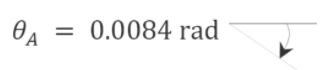
Deflection of beams through geometric methods: The geometric methods considered in this chapter includes the double integration method, singularity function method, moment-area method, and conjugate-beam method. Prior to discussion of these methods, the following equation of the elastic curve of a beam was derived:

Method of double integration: This method involves integrating the equation of elastic curve twice. The first integration yields the slope, and the second integration gives the deflection. The constants of integration are determined considering the boundary conditions.

Method of singularity function: This method involves using a singularity or half-range function to describe the equation of the elastic curve for the entire beam. A half-range function can be written in the general form as follows:

\(\langle x-a\rangle^{n}=\left\{\begin{array}{c}
0 \text { for }(x-a)<0 \text { or } x<a \\
(x-a)^{n} \text { for } x-a \geq 0 \text { or } x \geq a
\end{array}\right.\)

The method of singularity is best suited for beams with many discontinuities due to concentrated loads and moments. The method significantly reduces the number of constants of integration needed to be determined and, thus, makes computation easier when compared with the method of double integration.

Moment-area method: This method uses two theorems to determine the slope and deflection at specified points on the elastic curve of a beam. The two theorems are as follows:

First moment-area theorem: The change in slope between any two points on the elastic curve of a beam equals the area of the \(\frac{M}{E I}\) diagram between these two points.

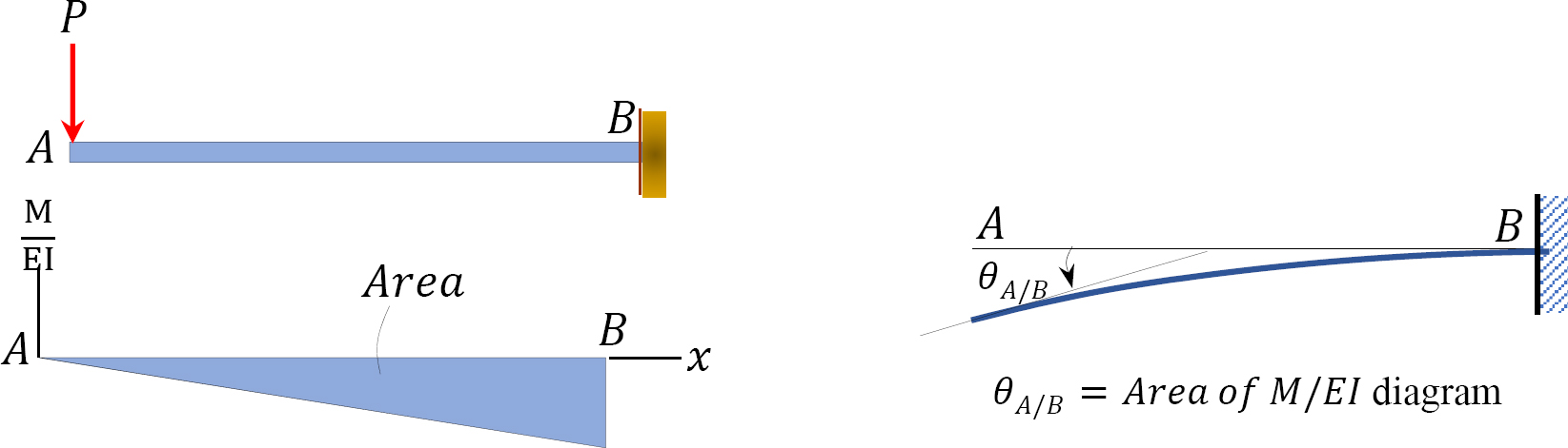
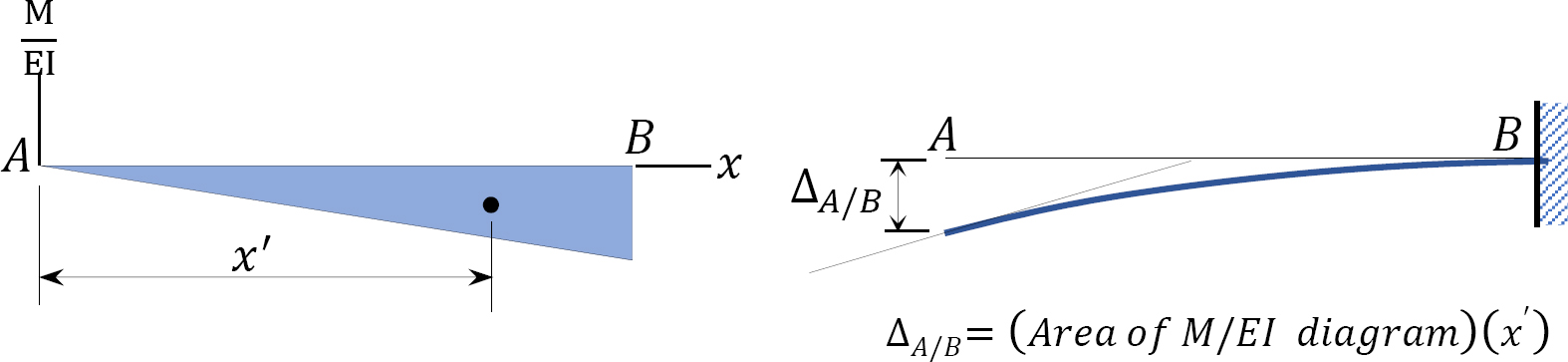
Second moment-area theorem: The vertical deflection of point \(A\) from the tangent drawn to the elastic curve at point \(B\) equals the moment of the area under the \(\frac{M}{E I}\) diagram between these two points about point \(A\).

Conjugate beam method: A conjugate beam has been defined as an imaginary beam with the same length as that of the actual beam but with a loading equal the \(\frac{M}{E I}\) diagram of the actual beam. The supports in the actual beams are replaced with fictitious supports with boundary conditions that will result in the bending moment and the shear force at a specific point in a conjugate beam equaling the deflection and slope, respectively, at the same points in the actual beam.

Practice Problems

7.1 Using the double integration method, determine the slopes and deflections at the free ends of the cantilever beams shown in Figure P7.1 through Figure P7.4. \(EI\) = constant.

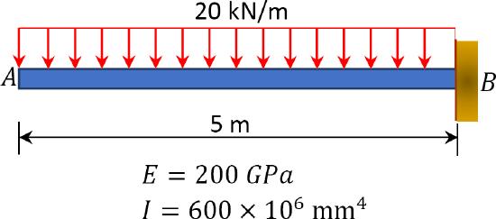
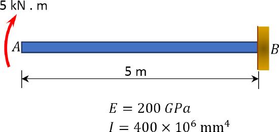
\(Fig. P7.1\). Cantilever beam.

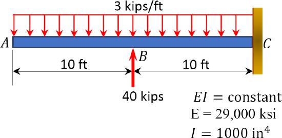
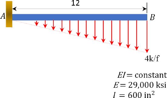
\(Fig. P7.2\). Cantilever beam.

\(Fig. P7.3\). Cantilever beam.

\(Fig. P7.4\). Cantilever beam.

7.2 Using the double integration method, determine the slopes at point \(A\) and the deflections at midpoint \(C\) of the beams shown in Figure P7.5 and Figure P7.6. \(EI\) = constant.

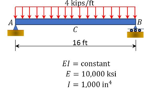
\(Fig. P7.5\). Beam.

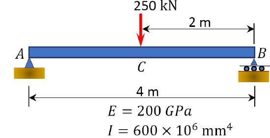
\(Fig. P7.6\). Beam.

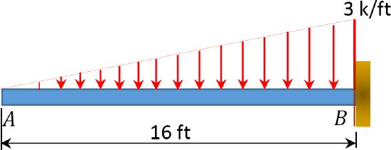
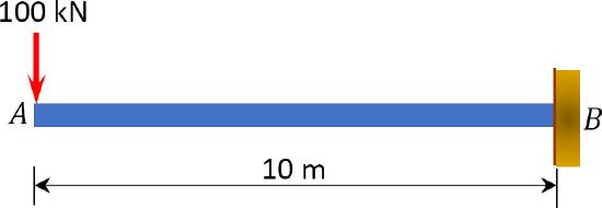
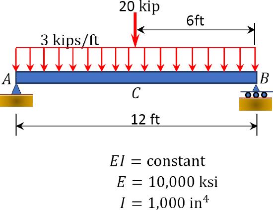
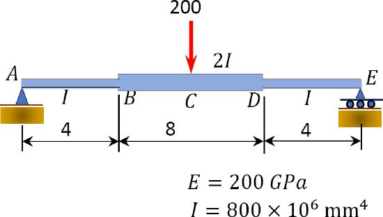
7.3 Using the conjugate beam method, determine the slope at point \(A\) and the deflection at point \(B\) of the beam shown in Figure P7.7 through Figure P7.10.

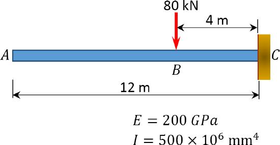
\(Fig. P7.7\). Beam.

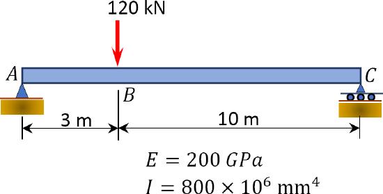
\(Fig. P7.8\). Beam.

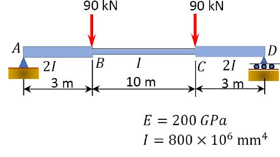
\(Fig. P7.9\). Beam.

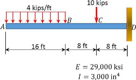
\(Fig. P7.10\). Beam.

7.4 Using the moment-area method, determine the deflection at point \(A\) of the cantilever beam shown in Figure P7.11 through Figure P7.12.

\(Fig. P7.11\). Cantilever beam.

\(Fig. P7.12\). Cantilever beam.

7.5 Using the moment-area method, determine the slope at point \(A\) and the slope at the midpoint \(C\) of the beams shown in Figure P7.13 and Figure P7.14.

\(Fig. P7.13\). Beam.

\(Fig. P7.14\). Beam.

7.6 Using the method of singularity function, determine the slope and the deflection at point \(A\) of the cantilever beam shown in Figure P7.15.

\(Fig. P7.15\). Cantilever beam.

7.7 Using the method of singularity function, determine the slope at point \(B\) and the slope at point \(C\) of the beam with the overhang shown in Figure P7.16. \(EI\) = constant. \(E=200 \mathrm{GPa}, \mathrm{I}=500 \times 106 \mathrm{~mm}^{4}\).

\(Fig. P7.16\). Beam.

7.8 Using the method of singularity function, determine the slope at point \(C\) and the deflection at point \(D\) of the beam with overhanging ends, as shown in Figure P7.17. \(EI\) = constant.

\(Fig. P7.17\). Beam.

7.9 Using the method of singularity function, determine the slope at point \(A\) and the deflection at point \(B\) of the beam shown in Figure P7.18. \(EI\) = constant.

\(Fig. P7.18\). Beam.